Appendix B
Does Form Imply Function?
Data-processing Inequality
The data-processing inequality can be used to show that no clever manipulation of the data can improve the inferences made from that data (see for more detail [61]).
Definition
Random variables are said to form a Markov chain if the conditional distribution of depends only on and is conditionally independent of . Specifically, form a Markov chain if the joint probability can be written as:
Theorem
(Data-processing inequality) If , then .
Proof: By the chain rule, the mutual information can be expanded in two different ways:
(B.2)
Since and are conditionally independent given , we have . Conversely, if , this would give
Thus we only have equality if and only if for Markov chains. Similarly, one can prove that .
Corollary
If
Proof: forms a Markov chain .
This result implies that no function can increase the information about .
Corollary
If , then
From eq. (B.2) it is noted that due to the definition the Markov chain and . Therefore:
The dependence of and is decreased or remains unchanged by the observation of a “downstream” random variable . For any complex system in which the state distribution follows a Markov chain, i.e. . The mutual information will always decay to zero as .
A Note on Causality and Mutual Information
Mutual Information and Causal Bivariate Interaction
Mutual information decays to causal interactions for simple bivariate interactions. For Markovian systems, the future state of the system is independent of its past given its present (eq. (2.2)). Therefore, we can write ([61])
(B.5)
For any two nodes , the KL-divergence reduces to .
Theorem
when and have no common neighbors.
Proof:
(B.6)
Mutual Information and Time Symmetry
The methods applied in the main text imply that the metric can be used symetrically. In this study time-delayed mutual information was performed in a ‘forward’ manner for pratical purposes. Namely, the system state was simulated for positive from some . For undirected networks there is a symmetry with regard to where information flows. Information is not bounded by any directionality of edges (fig. B.II.1b).
It is important to emphasize that this (generally) is not the case for directed networks. For kinetic Ising models detailed balance is not guaranteed and as such mutual information may be conflated for integrated nodes (see B.II). If information is constricted to flow in one direction, the mutual direction of time simulation is crucial. Additionally, directed networks show that the metric can be applied for different purposed. This can be seen in fig. B.II.1a, where forward simulations gives ‘information sinks’ and backward simulation provides ‘information sources’. IMI in directed networks will provide information about what nodes receive the most information over time, i.e. the correlation of a node with “sending” information. In contrast, simulating backwards shows what nodes have most impact on the instantaneous state of the system. This dual-use of information will be the focus of future studies.
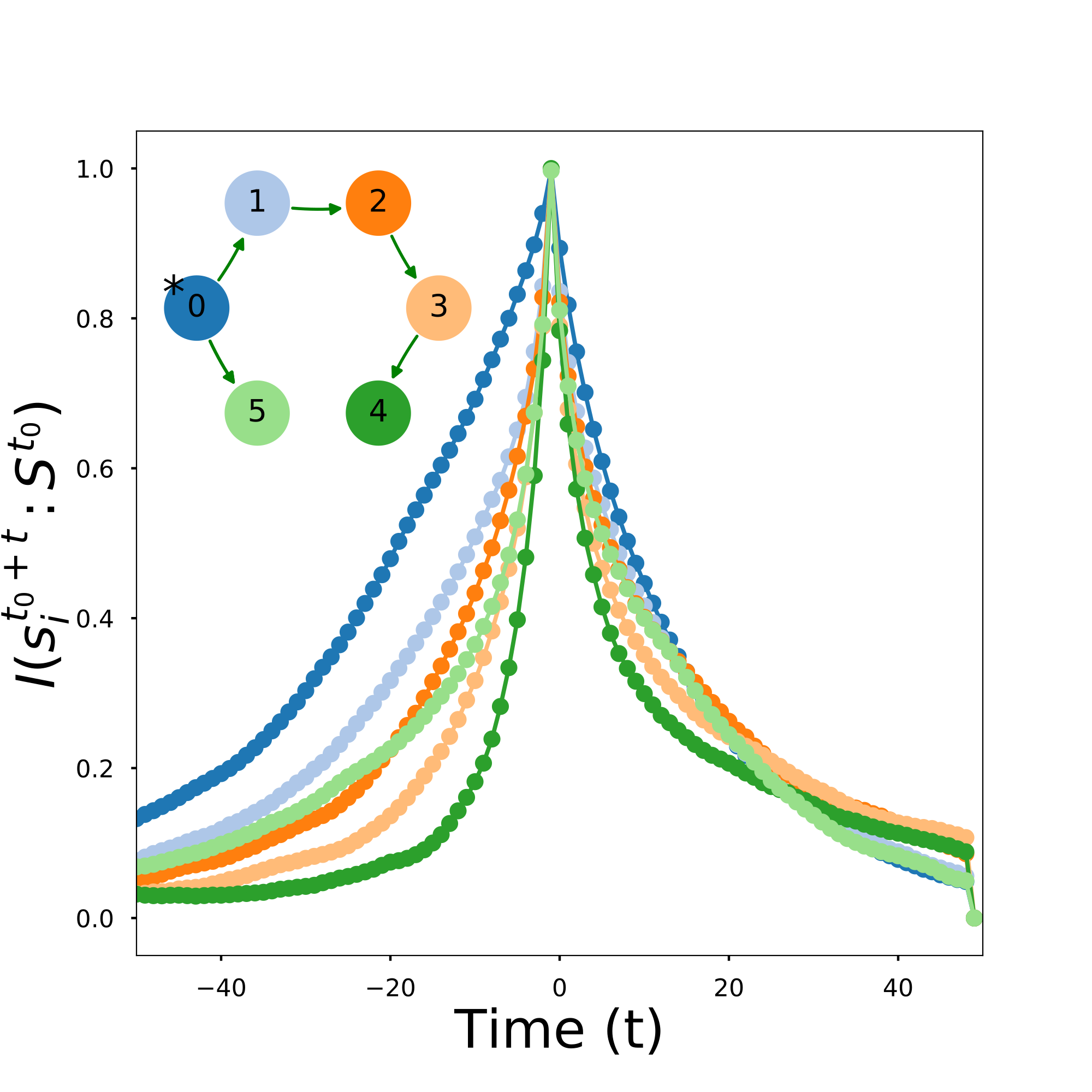
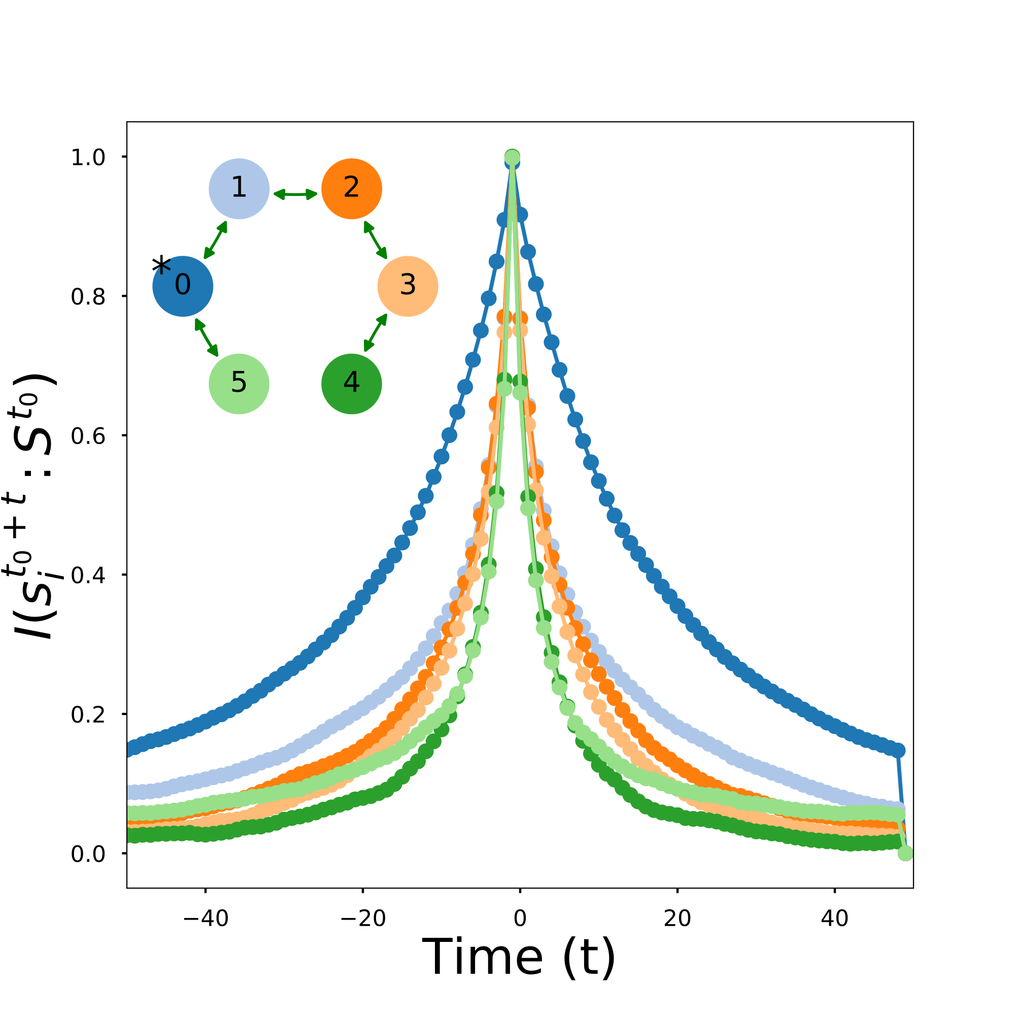
figure B.II.1b shows that for undirected networks there is no difference between node importance before or after ; information flows both directions.
Integrated Mutual Information and Integrator nodes
As noted in B.II the driver node can only be determined for ergodic systems with symmetric edges, that is the interaction . For directed graphs (i.e. non-symmetric edge weights) integrated mutual information may be conflated and produce a wrong estimate for the driver node. These cases are, however, outside the scope of the manuscript, and undirected integrators can readily be identified by integrated mutual information.
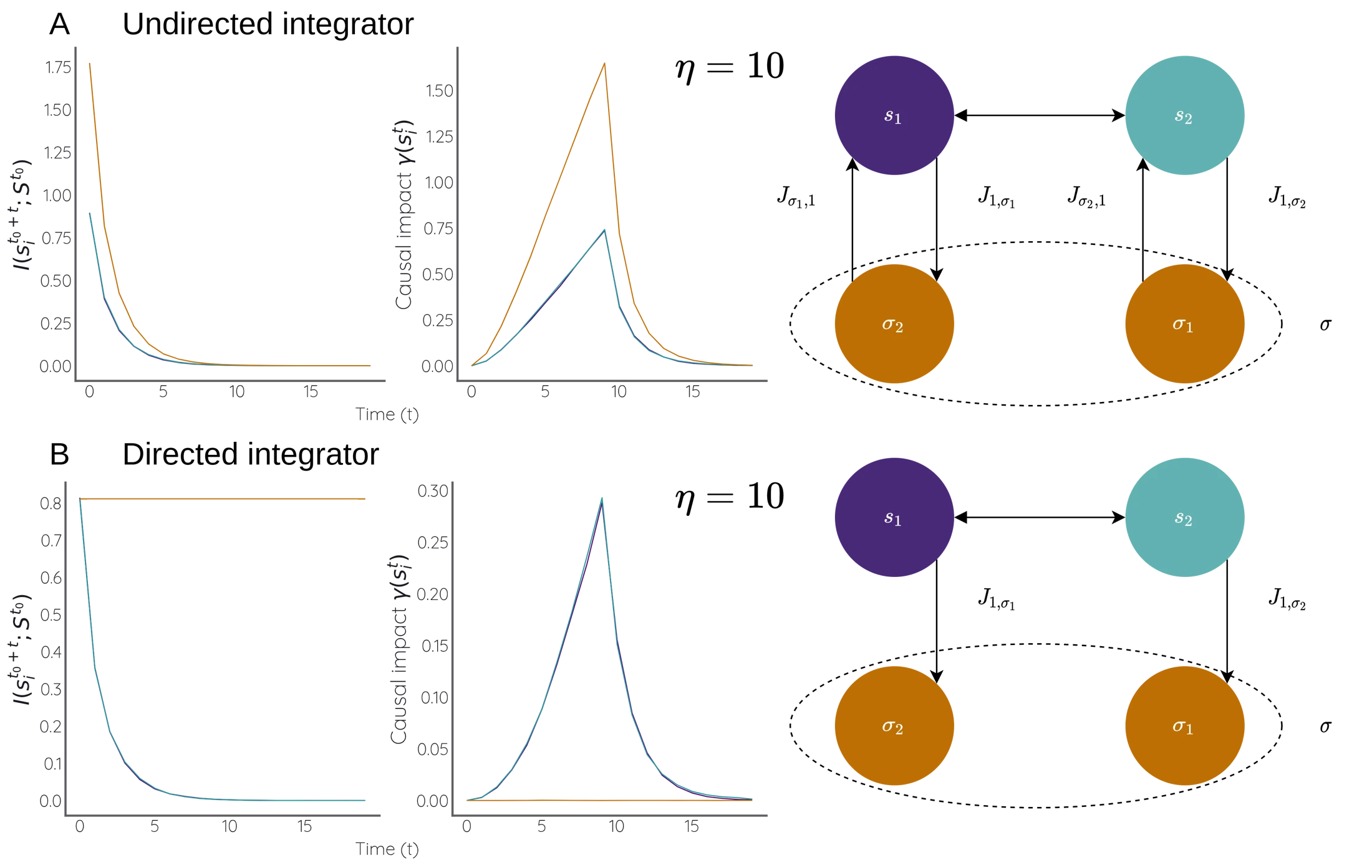
Consider the system where integrator with , and each node is governed by kinetic Ising spin dynamics (see figure B.II.2). The node is the integrator node that consists of two “sub-nodes” that connects to node separately. Note that the interaction weight can be adjusted. The traditional kinetic Ising spin dynamics are obtained for we obtain the traditional kinetic Ising spin dynamics, and as the dynamics tend to a copy operator. In addition, the weights may be set such that a directed graph is obtained (see figure B.II.2 B).
We consider two cases. First the case where contains no outgoing causal connections, that is . In the extreme case where the integrator is a copy operator (), the integrator stores information the system, but has itself no causal impact. Integrated mutual information in this setting cannot be used as a driver node identification as the shared mutual information with the system is merely correlational.
For undirected edges, however, e.g. (fig B.II.2 A), integrator node will have the highest causal potential as the impact of an intervention on the integrator can percolate through the system. Integrated mutual information correctly identifies the driver node. Note that the size of the connection weights matters. As the interaction the integrator node will tend to a copy operator. For a copy operator the dynamics of the system will degenerate. In this setting, the out-of-equilibrium dynamics will be non-existing as the dynamics of and will be frozen through the edge with the integrator. This will results that out-of-equilibrium, the system state will merely be copied and no transient dynamics will be possible. Information flows will not occur as the relative entropy will be zero. This setting violates detailed balance. Relaxing the interaction , enables detailed balance and we see under these conditions the driver node is correctly identified (fig. B.II.2 A). The integrator node’s causal impact can flow due to the detailed balance.
In conclusion, directed edges violates detailed balance and consequently integrated mutual information will not be able to identify the driver node as the node with the highest mutual information through forward inference, i.e. ). Nodes with the highest causal impact are correctly identified through integrated mutual information for kinetic Ising spin dynamics on undirected network structures where detailed balance is ensured.
Time Reversibility and Detailed Balance
In order to show that , we have to show that .
Two-sided Markov Chains
For a positive recurring Markov chain with transition matrix and stationary distribution , let a stationary version of this chain, i.e. . We can construct a two-sided extension of by defining a shift , extending the process backwards in time: with . It is true that by stationarity has the same stationary distribution as : we arrive at .
Detailed balance
Let be a two-sided extension of a positive recurrent Markov chain with transition matrix and stationary distribution . A transition from state to is denoted with notation .
In other words the time-reverse Markov chain is a Markov chain with transition probabilities:
This is also known as detailed balance. In the manuscript, ergodic systems are used and therefore satisfy the time-symmetry. This results that .
Data Correction and Fit Errors
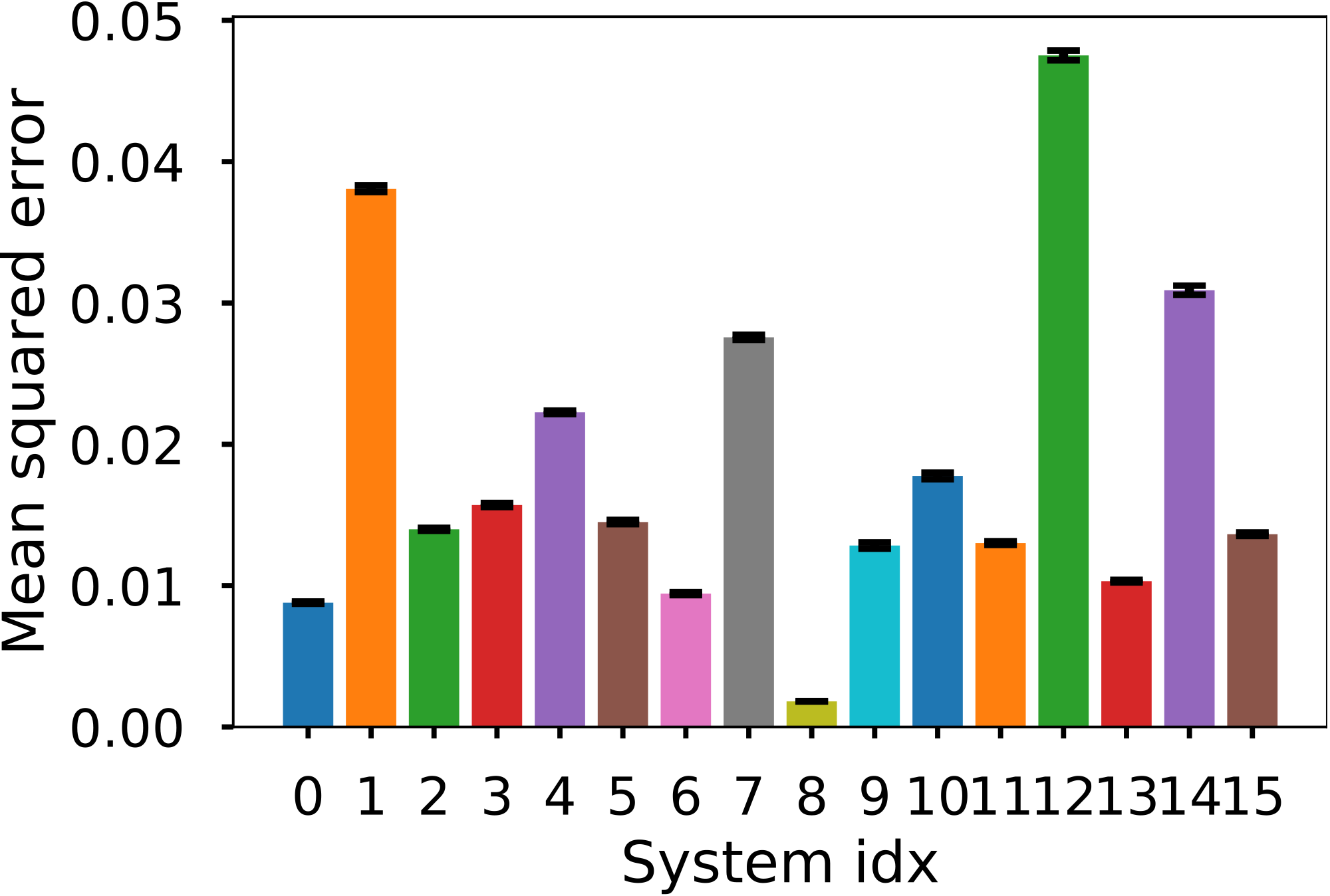
To assess the accuracy of the Monte-Carlo simulations, we evaluated the model fit using mean-squared error. Double exponentials were fitted to estimate the curves before computing the are aunder the curve. For both the the random graphs and the psychosymptom system, the mean squared error was calculated. The results are shown in Figure B.III.1a and Figure B.III.1b.
Validation of Psychosymptoms
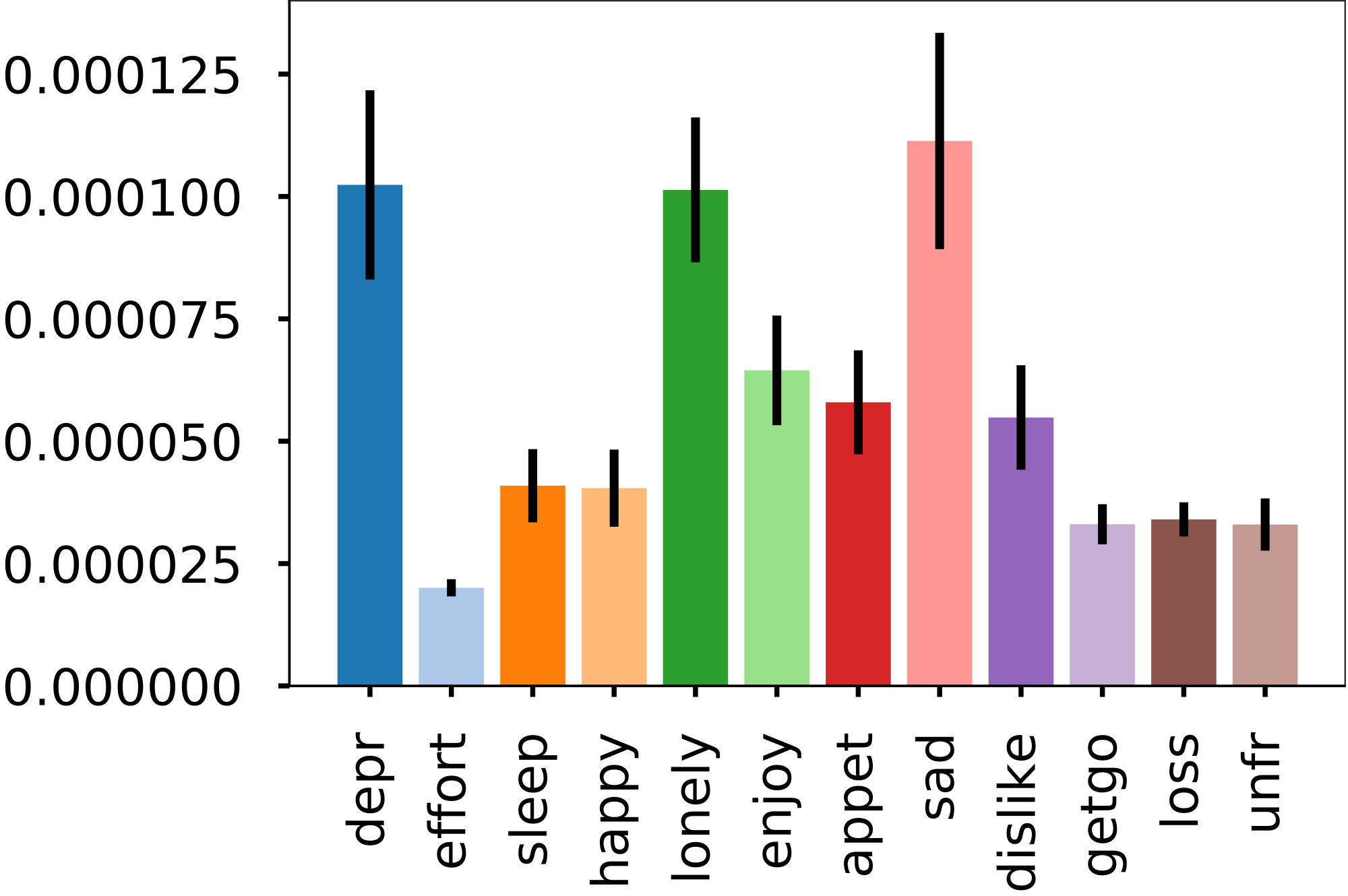
The results from this study imply that for low thermal noise not enough resolution was possible to reliably estimate the driver node. For medium to high noise levels, the ‘sad’ emerged as the driver node.
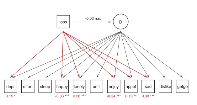
In the original study, the bereavement score was most affected by ‘lonely’, and showed weak negative associations with ‘happy’ and ‘effort’ (fig. B.IV.1 adopted from [86]). Consequently, it seems that medium to high thermal noise is most congruent with the original study. Fried and colleagues postulated that ‘lonely’ was the gateway from which information spreads through the network, i.e. bereavement was embodied mainly by ‘loneliness’ which then percolated its effect to the other symptoms. Since the nature of the data was cross-sectional, the comparison with the results from this study relies on the assumption that binary dynamics are representative of the absence and presence of psychological symptoms. If correct, the results from this study give a causal perspective on the associative results from [86]. The results from this study postulate that ‘depr’, ‘lonely’ and ‘sad’ have similar causal effect for moderate to high thermal noise.
It is important to emphasize that a quantification is given in terms of absolute effect size and not directed effects. This means that nudging for instance ‘sleep’ has some effect on the psycho-symptom network, in what direction that effect is, or whether it has a positive or negative effect on the bereavement score / cognitive load of the patient is not clear, and should be the subject of future studies.
As a final note, the field of psychometrics is concerned with relating how observables (e.g. behavior, responses on questionnaires, etc) relate to theoretical cognitive constructs such as intelligence or mental disorders. A common approach in understanding high level phenomena such as depression is to use a latent variable model, i.e. assuming some high abstract feature to be the cause of the observables (or vice versa). Only recently has this paradigm shifted from a latent variable model to a network based approach [59], [214], [215]. Marsman et al. recently reconciled these two approached by showing statistical equivalence between the Ising model and canonically used latent variable models in psychometrics [216]. The two approaches thus highlight different aspects in theory building; measurement invariance and correlation structure may be interesting from a common cause approach but not from a network perspective which is more interested in dynamical aspects of the system. Both approaches, however, aid in highlighting different aspects of the psychological constructs.
Code Manual
Accompanying this paper, we developed a general framework for analyzing discrete systems using IMI. The code is written in python 3.7.2 and uses cython 0.28.2 for c/c++ level performance. The code is freely available on cvanelteren.github.ioincludes the latest build instructions.hat follows here is a brief overview of the framework.
Structural Methods
Network analysis has traditionally resulted in analyzing the structure of the network. A fundamental concept within network science is centrality, and how to measure the centrality of nodes has become an essential part of understanding networked systems such as social networks, the internet, biological networks, traffic and ecological networks. At its core, a centrality measure quantifies the ‘importance’ of a node based on some structural property. It allows ranking nodes based on a real-valued function.
There is, however, a long-standing debate concerning what centrality metrics actually measure for networked systems [51], [91], [92], [217] . From a network theoretical perspective most centrality measures, e.g. betweenness, closeness, eigenvector and degree centrality, essentially classify the ‘walk structure’ of a network [91], [92]. A walk from node to node is a sequence of adjacent nodes that begins with and ends with . The structure of walks can be divided along different criteria. For example a trail is a walk in which no edge (i.e. adjacent pair of nodes) is repeated. In contrast, a path is a trail in which no node is visited more than once. Similarly, one could define a walk structure by only using the shortest path from one node to another, or by using random movements between nodes (random walks).
Alternatively, from a complex systems perspective, centrality metrics implicitly assume dynamics on the network structure. Betweenness centrality for example, computes centrality based on how often a node acts as a bridge along the shortest path between two other nodes. If one assumes that the network has dynamics where information between nodes follows the shortest path, this metric may be a valid description to use and identify dynamically important nodes.
In the best case, a centrality metric is fully predictive for identifying important nodes a complex system. Consequently, the centrality metric can be used to understand the system. However, an issue with the use of centrality metrics is determining which centrality metric to use. Consider for example figure Figure 2.1; different centrality metrics can identify different nodes as most central. This has lead to the common observation that some centrality measures can ‘get it wrong’ when the aim is to predict dynamical important structure in networked systems. Additionally, the ranking produced through some centrality metric does not quantify inter-rank differences. This potentially leads to underestimation of nodal influence when used in dynamic context [51].
We will show how centrality measures have no meaningful prediction power of the most causal node in nodes dictated by the Gibbs measure. We are aware that centrality measures do not embody the full extent of what structural methods embody, or what network science in particular has to offer. However, many structural methods share the common characteristics listed above, i.e. they quantify the walk structure of a network. For our analysis, we used the weighted variants of degree centrality, betweenness centrality, information centrality, and eigenvector centrality. What follows is a brief description of commonly used centrality metrics.
Degree Centrality
Degree centrality is the best-known measure of all the centrality measures. It is often thought that degree centrality is indicative for the dynamic importance of a node. This intuition is based on the concept of flow: the more connection a node has, the more interaction potential that node has and therefore the more important a node must be. Freeman defined centrality measure as the count of the number of edges incident upon a given node [218]:
(B.9) where is the row/column of node in the adjacency matrix of the network. Please note that the entries are weighted and not binary.
Betweenness Centrality
Betweenness centrality quantifies the number of times a node acts as a bridge along the shortest path between two other nodes. It was introduced as a measure for quantifying the control of communication among humans in social networks by Freeman [218]. Nodes that have a high probability to occur on a randomly chosen shortest path between two randomly chosen vertices have a high betweenness. Formally, this can be written as:
(B.10)
where represents the number of shortest paths between node and , and is the subset that goes through node . We use the normalized version of betweenness that divides the betweenness score by the number of pairs of vertices (not including node );
(B.11)
Closeness Centrality
Closeness centrality is defined as the reciprocal sum of the length of the shortest paths between the node and all other nodes in the network :
(B.12) From a complex system perspective it assumes that information is transferred along its shortest paths. A node with short distance to many other nodes will be able to quickly transfer its information to other nodes in the network.
Eigenvector Centrality
Eigenvector centrality is the most difficult centrality measure to give an intuitive feeling for. Where is the adjacency matrix of the system, eigenvector centrality of node is defined as:
(B.13)
For any square matrix of rank , the matrix will have at most eigenvector-eigenvalues pairs. A common choice for eigenvector centrality is motivated by The Perron-Frobenius theorem, and involves choosing the eigenvector with the largest eigenvalue [219], [220]. This has the desired property that if is irreducible, or equivalently if the network is strongly connected, that the eigenvector is both unique and positive.
The sign and size of the eigenvalue are important for the relation between the value and importance of a node. In linear differential equations negative eigenvalues correspond to non-oscillatory exponentially stable solutions. In contrast, in difference equations it indicates an oscillatory behavior. Geometrically speaking, negative eigenvector embodies a linear transformation across some axis.
Intuitively speaking, eigenvector centrality quantifies the influence of a node in the network. It assigns relatives scores to all nodes in the network based on the concept that connections to high-scoring nodes contribute more to the score of the node in question than equal connections to low-scoring nodes. A high eigenvector score implies that the node is connected to many other nodes that themselves have high scores. Google PageRank and Katz centrality are variants of eigenvector centrality [221]. A node with high eigenvector centrality is not necessarily a node that has many connection (incoming or outgoing). For example a node may have a high eigenvector centrality if it has few connections, but those connections are connected to nodes that are of high importance.
Bootstrap Distributions
A total of bootstrap samples were conducted with replacement. For each nodal bootstrap distribution a gaussian kernel density was estimated. The node with the highest causal impact was chosen as the initial driver set . Then the overlap between this driver node and the remaining nodes in the system was computed iteratively. We considered the overlap or higher was sufficient for the node was to be considered causally similar to the driver node. Therefore, the proposed node will be included in the driver node set if . We will first outline the procedure after which we discuss the results from this procedure.
Numerical Procedure
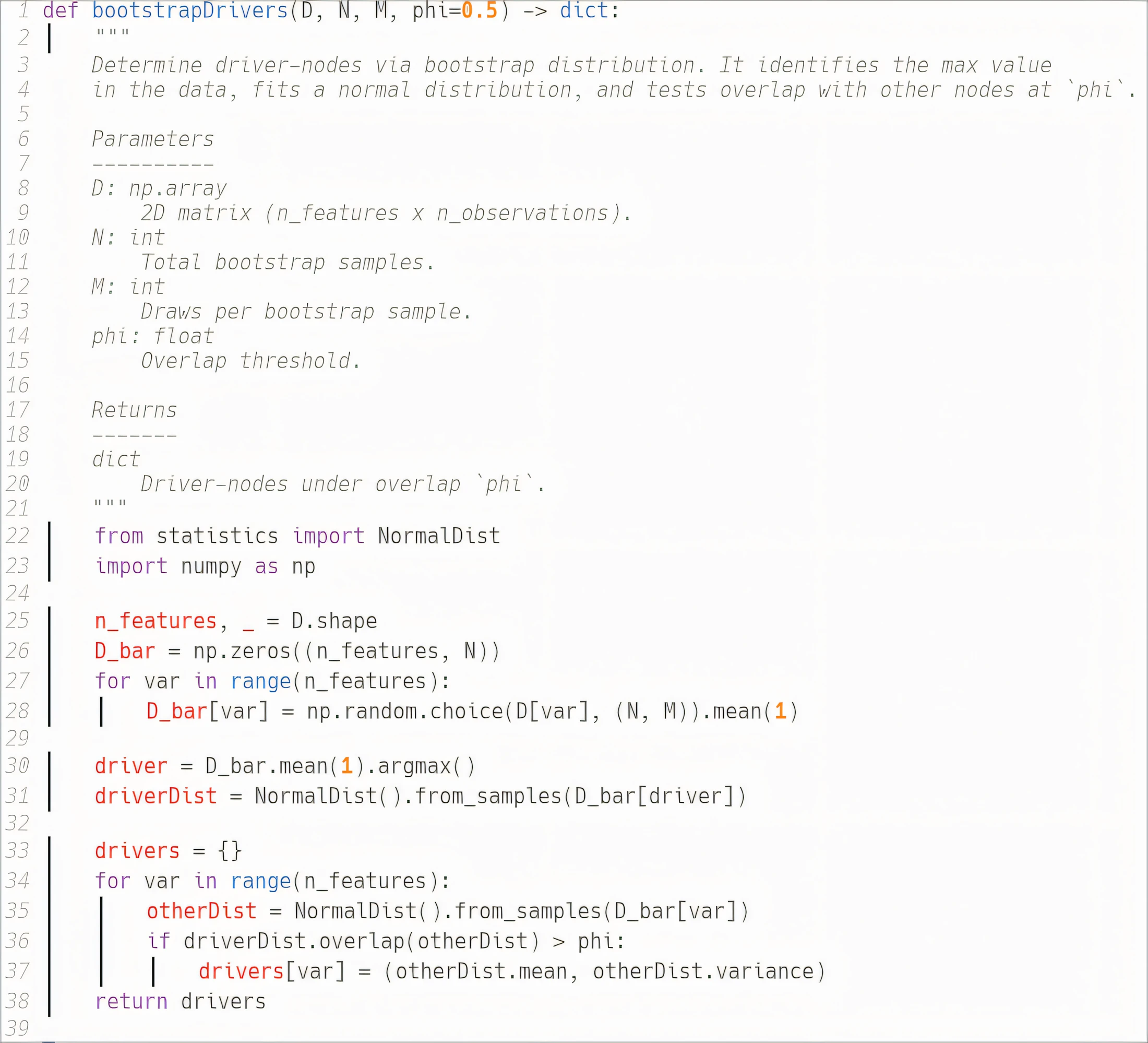
The driver node detection algorithm is implemented in Python, with its core functionality illustrated in Algorithm B.VII.1. The algorithm employs a bootstrap-based approach to identify driver nodes through iterative distribution analysis. Starting with a data matrix of features and observations, the procedure generates bootstrap samples and fits normal distributions to analyze the relationships between nodes.
The algorithm first identifies the node with the highest mean value across bootstrap samples as an initial driver. Subsequently, it evaluates other nodes by comparing their distributions with the driver node’s distribution using an overlap criterion . Nodes whose distributions overlap significantly with the driver (above the threshold ) are included in the driver set. Algorithm B.VII.1 provides a visual representation of the algorithm’s workflow, demonstrating the bootstrap sampling and distribution comparison processes.
This implementation leverages Python’s standard library components, specifically the statistics module for normal distribution calculations, ensuring computational efficiency and statistical robustness. The method is particularly effective for analyzing complex systems where traditional deterministic approaches might be insufficient.
Erdős-Rényi Networks
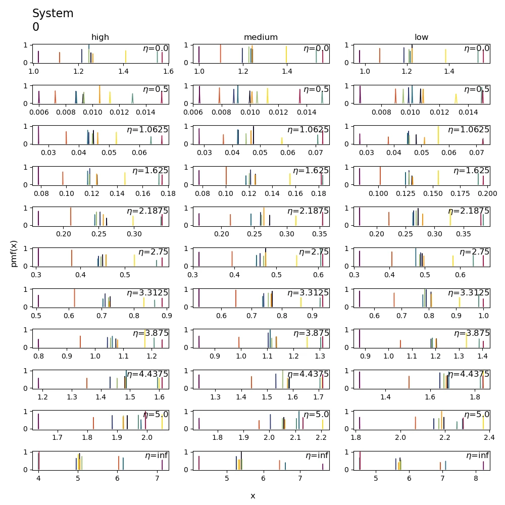
Bootstrap distributions using kernel density estimates are illustrated for Erdős-Rényi networks in Figure B.VII.2. The x-axis represents the area under the curve for either integrated mutual information () or causal impact (), where indicates the area under the curve for either causal impact or integrated mutual information. A representative distribution from system 0 is shown here, as the distributions across different systems exhibit similar characteristics. The complete set of bootstrap distributions for all experimental conditions, including additional network configurations, can be found in the supplementary materials of [45].
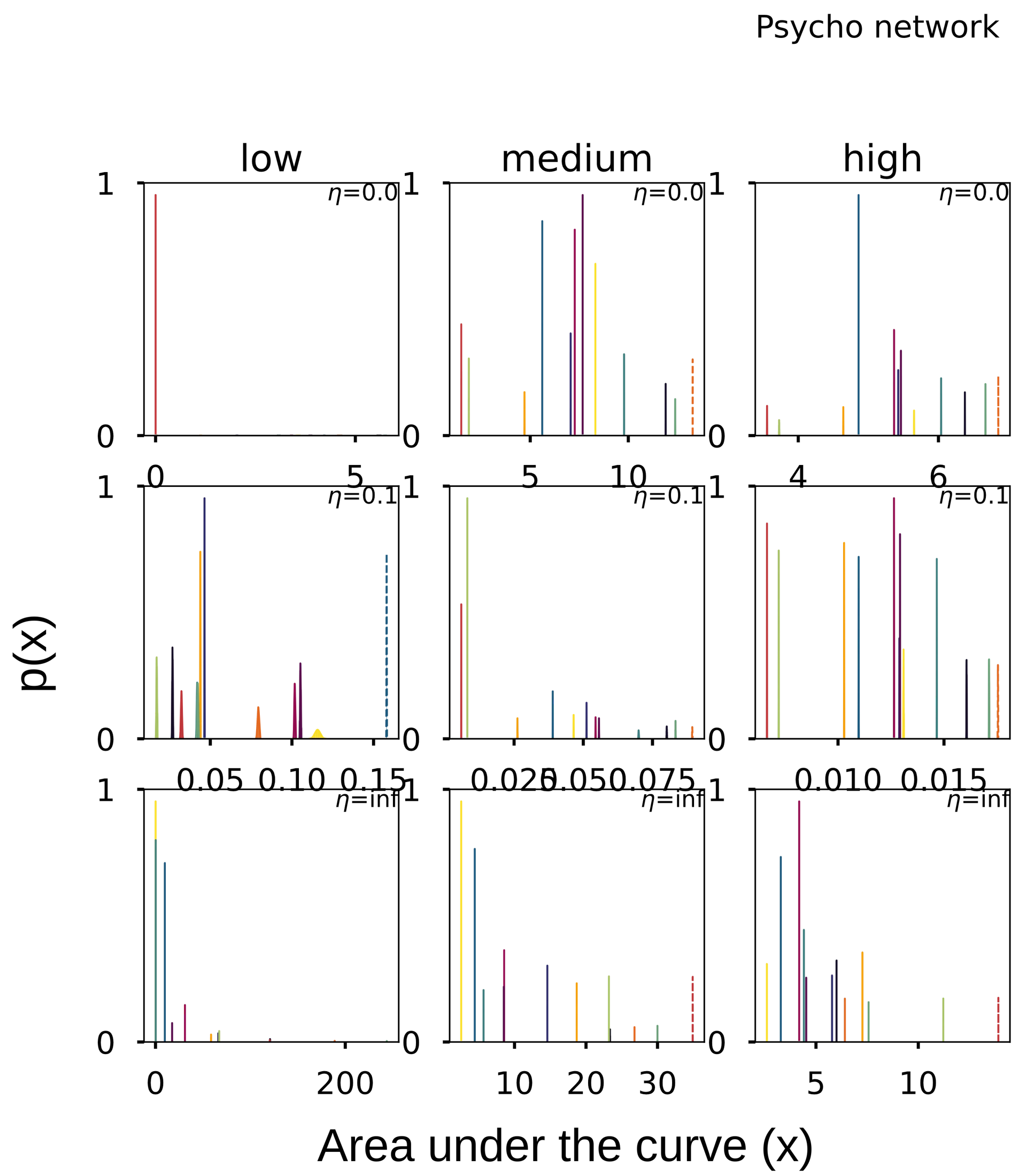
Psycho Networks
Note here refers to the input variable which are the area under curves either for integrated mutual information () or for causal impact .
Software
A general toolbox was developed for analyzing any discrete systems using IMI, e.g. Susceptible-Infected-Recovered [222], Random Boolean networks [223]. The core engine is written in 3.07a with python 3.9.4 and offers C/C++ level performance1, for more information see https://github.com/cvanelteren/information_impact.