Does function imply form?

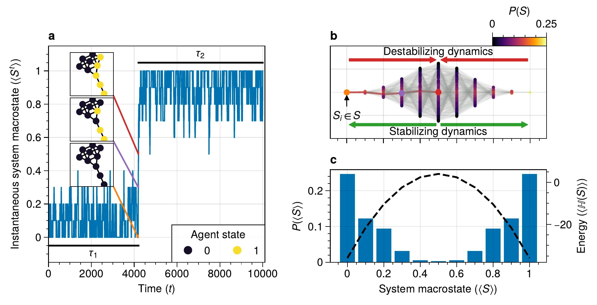
While our previous exploration revealed the limitations of inferring dynamic importance from structural features alone, we now delve into a phenomenon that further complicates the form-function relationship in complex systems: multistability. This crucial characteristic, observed in various real-world complex systems [1], [94], presents another layer of complexity in understanding how function shapes and is shaped by form. Multistability describes the phenomenon in which a system explores different states within its state space at various spatio-temporal scales.

Evidence increasingly suggests that noise fluctuations play a fundamental role in these transitions between attractor states [95], [96], [97]. Traditionally, noise is perceived as an unwanted signal, diminishing system effectiveness or signal quality. However, in nonlinear systems, such as interconnected neurons in the brain, noise can play a surprising role by enabling the exploration of larger parts of the state space, allowing the system to escape local minima [98], [99].

This understanding of noise-induced transitions has enriched our classical view of multistability. While multistability has historically been studied from an equilibrium perspective [98], [100], [101], recent research has revealed how network structure fundamentally affects both the stability of these states and the pathways between them [3], [5], [102], [103].

The challenge of understanding and controlling these network transitions has been approached from multiple angles. Recent work has utilized algorithmic information theory to measure the computational complexity of producing network states through controlled interventions [104], [105], [106]. While this provides powerful tools for steering networks through external manipulation, fundamental questions remain about how networks spontaneously transition between states through their internal dynamics. Our approach uses Shannon information theory to quantify the temporal correlations that emerge naturally as networks evolve, revealing how noise propagates through network structure to generate endogenous transitions. This complements algorithmic approaches by focusing on the statistical mechanisms underlying spontaneous state changes rather than the computational complexity of producing specific states.

To address these fundamental questions about noise-induced transitions, this chapter focuses on a critical gap in our understanding of networked dynamical systems out of equilibrium. We focus on systems where each node’s state evolves according to the Boltzmann-Gibbs distribution, a framework applicable to various phenomena including neural dynamics [107], opinion formation, and ferromagnetic spins [89].

The analysis reveals two key classes of nodes that mediate these transitions. Firstly, we introduce the concept of initiator nodes, which play a fundamental role in propagating noise within the system. These initiator nodes serve to destabilize nodes occupying lower energy states, thereby priming the system towards a transition. As the transition initiates, a cascade of flips is rapidly triggered by these initiator nodes, propelling the system towards a new metastable state. Secondly, we identify the significance of stabilizing nodes in counteracting the effects of noise and maintaining the system in a metastable state. These nodes act to stabilize the system amidst the disruptive influence of noise, thereby contributing to the persistence of the metastable state.

To quantitatively characterize the roles of these nodes and their interactions, two novel information theoretic measures were introduced (Chapter 2). These measures, namely integrated mutual information and asymptotic information, are designed to capture the effects of short-term and long-term correlations, respectively. They provide valuable insights into the dynamics of metastable transitions within networked systems and can be directly computed from observations.

Integrated mutual information captures the transient destabilization of the system, revealing the role of initiator nodes in triggering systemic transitions. Asymptotic information, on the other hand, quantifies the long-term memory encoded by stabilizer nodes, which ultimately reverse the domino effect and settle the network into a new stable attractor. By manipulating these roles, we demonstrate how targeted interventions can either promote or inhibit systemic transitions, offering a new approach to controlling critical transitions in complex networks.

The computational method uncovers a network percolation process that facilitates noise-induced transitions without external parameter changes, offering a fresh perspective on tipping points in complex networks [108], [109], [110], [111]. This approach bridges the gap between local equilibrium dynamics and global system behavior, providing insights into how network structure influences systemic transitions [3], [5], [112], [113], [114].

By revealing the the domino-like mechanisms of endogenous state transitions, the work has broad implications for predicting and potentially controlling critical transitions in diverse complex systems. From enhancing brain plasticity to anticipating ecosystem shifts, this framework provides a foundation for understanding and managing multistability in an interconnected world.

Noise-Induced Transitions

We focus on dynamical systems where the state transitions of individual nodes are governed by the Boltzmann-Gibbs distribution. This distribution, fundamental in statistical mechanics, provides a probabilistic framework for describing the behavior of systems in thermal equilibrium. In this context, it determines the likelihood of a node transitioning from one state to another based on the energy difference between states and a global noise parameter. Specifically, the probability of a node transitioning from state $s_i$ to state $s_i'$ is given by: $$\begin{equation} P(s_i \to s_i') = \frac{1}{1 + \exp(-\beta \Delta E(s_i, s_i'))}, \end{equation}$$ where $\Delta E(s_i, s_i')$ represents the energy difference for the state transition, and $\beta$ is the inverse temperature or noise parameter. This formulation captures the essence of how local interactions and global noise influence state changes in the networked system. Higher values of $\beta$ correspond to lower noise levels, leading to more deterministic behavior, while lower $\beta$ values introduce more randomness into the system’s dynamics. This framework allows us to model a wide range of phenomena, from neural activity to opinion dynamics, within a consistent mathematical structure.

Fluctuations and their correlations at time $\tau$ are captured using Shannon’s mutual information [61] shared between a node’s state ($s_i^t$) at time $t$ and the entire future system state ($S^{t+\tau}$), $I(s_i^{\tau} : S^{\tau + t})$. The time lag $t$ is used to analyze two key features of information flows of a system: the area under the curve (AUC) of short-term information, and sustained level of long term information.

The contribution of a node to the dynamics of the system will differ depending on the network connectivity of a node (Figure C.V.1) [45], [75]. The total amount of fluctuations shared between the node’s current state and the system’s short-term future trajectory is computed as the integrated mutual information

$$\begin{equation} \begin{split} \mu(s_i) = \sum_{t = 0}^\infty (I(s_i^{\tau} : S^{\tau + t}) - \omega(s_i)) \Delta t. \end{split} \end{equation}$$(3.2)

Intuitively, $\mu(s_i)$ represents a combination of the intensity and duration of the short-term fluctuations on the (transient) system dynamics [45]. It reflects how much of the node state is in the “working memory” of the system.

The term $\omega(s_i) \in \mathbb{R}_{\ge 0}$ represents the system’s long-term memory. As the system transitions between stable points, short-lived correlations evolve into longer-lasting ones, particularly among less dynamic nodes. When $\omega(s_i)$ is positive, it indicates a separation of time scales: ephemeral correlations dissipate, giving way to slower, more persistent fluctuations. These enduring fluctuations reflect the multiple attractor states accessible to the system, with less dynamic nodes becoming more aligned with future system states.

Near a stable attractor, the system primarily generates short-lived fluctuations. However, as it approaches a tipping point, longer-lasting correlations emerge. These persistent correlations facilitate the system’s transition from one stable attractor to another, much like repeated nudges eventually push a ball over a hill. The asymptotic information, $\omega(s_i)$, quantifies this transition potential. Higher values of $\omega(s_i)$ indicate a greater likelihood of state transition, with the exact value reflecting each node’s contribution to the tipping behavior.

Asymptotic information distinguishes itself from other early warning signals—such as increased autocorrelation, critical slowing down captured by Fisher information, changes in skewness or kurtosis, and increased variance—by specifically measuring the system’s long-term memory and temporal correlation structure. While entropy captures the overall uncertainty or disorder in a system at a given moment, and mutual information quantifies the shared information between components at a particular time, asymptotic information focuses on the persistence of correlations over extended time periods. It reveals how past states influence future configurations, capturing aspects of the system’s dynamics that are not explained by instantaneous or short-term pairwise measures.

Using these information features, each node can be assigned to a different role based on their contribution to the metastable transition. We denote nodes with short-lived correlations as initiators pushing nodes towards a tipping point. In contrast, nodes with longer-lived correlations are referred to as stabilizers. For these nodes, their dynamics are less affected by short-lived correlations, and they require a higher mixing state for to transition from one state to another. The role assignment will be further discussed in 3.2.2.

We compute information flows using exact calculations on a randomly generated connected graph of $n=10$ nodes. The states are grouped based on their distance to the tipping point, defined as the energy barrier between two locally stable states. For the Ising model, this corresponds to the collection of states where $\langle S \rangle = 0.5$. We evaluate the conditional distribution up to $\tau = 300$ time steps.

This computational process scales exponentially with the number of nodes, $O(n) = 2^n$, which limits its applicability to large-scale systems without employing variable reduction techniques such as coarse-graining. Extending this analysis to larger systems will be the focus of future research.

For detailed replication instructions, please refer to Section C.

The Domino-Effect: A Balance Between Short-Lived and Long-Lived Correlations

The analysis reveals several key insights into the dynamics of metastable transitions and tipping points in complex networks. We observe a distinct domino effect where low-degree nodes initiate system destabilization. As the system approaches a tipping point, information flows shift from low-degree to high-degree nodes. we observe an increase in asymptotic information as a potential early warning signal for an impending tipping point. Finally, we uncover a division of roles among nodes, with some acting as initiators that propagate perturbations and others as stabilizers that influence the system’s transition between attractor states.

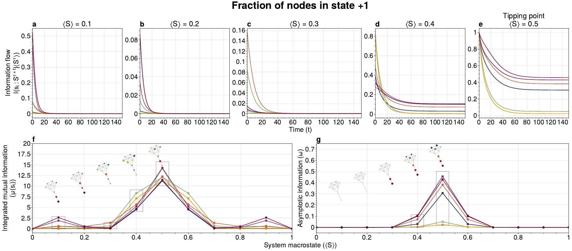
In Figure 3.2, we visualize the information flows at different stages as the system approaches the tipping point. While we present detailed analysis using the kite graph for simplicity, these findings generalize to other network structures, as demonstrated in Figure 3.5 and further elaborated in the appendix.

To decompose the metastable transition, we consider local information flows in a given system partition, $S_{\gamma} = \{S' \subseteq S | \langle S' \rangle = \gamma\}$ where $\gamma \in [0,1]$ represents the fraction of nodes having state 1. This yields the conditional integrated mutual information:

$$\begin{equation} \mu(s_i | \langle S \rangle) = \sum_{t = 0}^\infty (I(s_i^{\tau} : S^{\tau + t} | \langle S^{\tau} \rangle) - \omega_{s_i}) \Delta t. \end{equation}$$(3.3)

Details about the estimation procedure can be found in Appendix C.II.4.

Two key observations emerge from Figure 3.2:

Firstly, the tipping point is reached through a domino effect, with low-degree nodes acting as initiators early in the process. These nodes, being more susceptible to noise (see Figure C.V.1), are more likely to pass fluctuations to neighbors – akin to pushing a ball up a hill. Far from the tipping point (Figure 3.2a), lower-degree nodes show higher integrated mutual information, $\mu(s_i | \langle S \rangle)$, than higher-degree nodes. This noise injection by lower-degree nodes increases the likelihood of a metastable transition.

Secondly, an increase in asymptotic behavior corresponds to the system transitioning between attractor states. As shown in Figure 3.2(b, c), asymptotic information remains low far from the tipping point and steadily increases as the system approaches it. Nodes with higher asymptotic information possess greater predictive power regarding which side of the tipping point the system will settle on.

Path Analysis and Tipping Point Trajectories

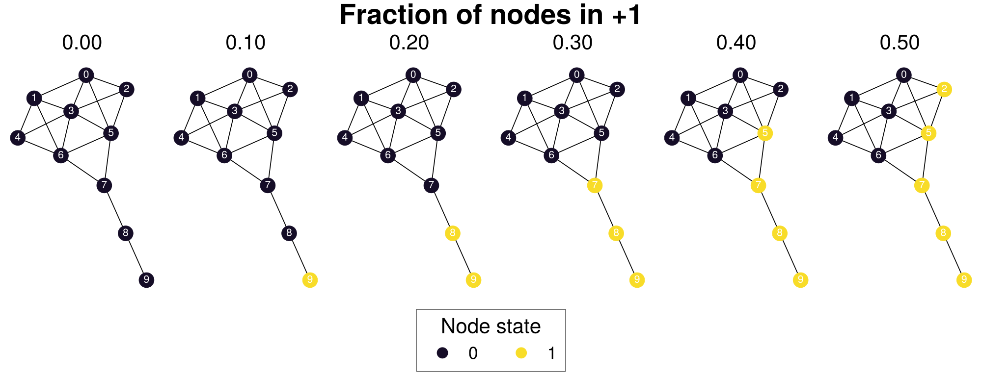
To illustrate the information encoded in these flows, we computed trajectories from the attractor state $S = \{0, \dots, 0\}$, simulated for $t=5$ steps. Figure 3.3 shows a trajectory that maximizes:

$$\begin{equation*} \log p\big(S^{t + 1}|S^{t}, S^0 = \{0, \dots, 0\}, \langle S^5 \rangle = 0.5\big). \end{equation*}$$(3.2.1)

These trajectories reveal how the information flows measured in Figure 3.2c are generated by the sequence of flips originating from the tail of the kite graph. Tail nodes are uniquely positioned to pass on fluctuations to their neighbors, eventually causing a cascade of flips that reach the tipping point. This simple example illustrates how the network structure can influence the system’s dynamics and the information flows that precede a metastable transition. Where noise pushes the system towards a tipping point, originating first in low degree nodes for dynamics governed by the Boltzmann-Gibbs distribution.

The domino effect is not solely determined by node degree. As the system nears the tipping point, network effects become significant. For instance, in the kite graph, node 8 (degree 2) exhibits the highest integrated mutual information when 2 bits are flipped (Figure 3.2b). In contrast, node 3 (degree 6) shows low shared information prior to the tipping point but high shared information at the tipping point.

This transition highlights how the network structure as a whole contributes to a system’s behavior. Local structural measures, such as degree centrality, may undervalue a node’s contribution towards a tipping point and the eventual settlement in a new attractor.

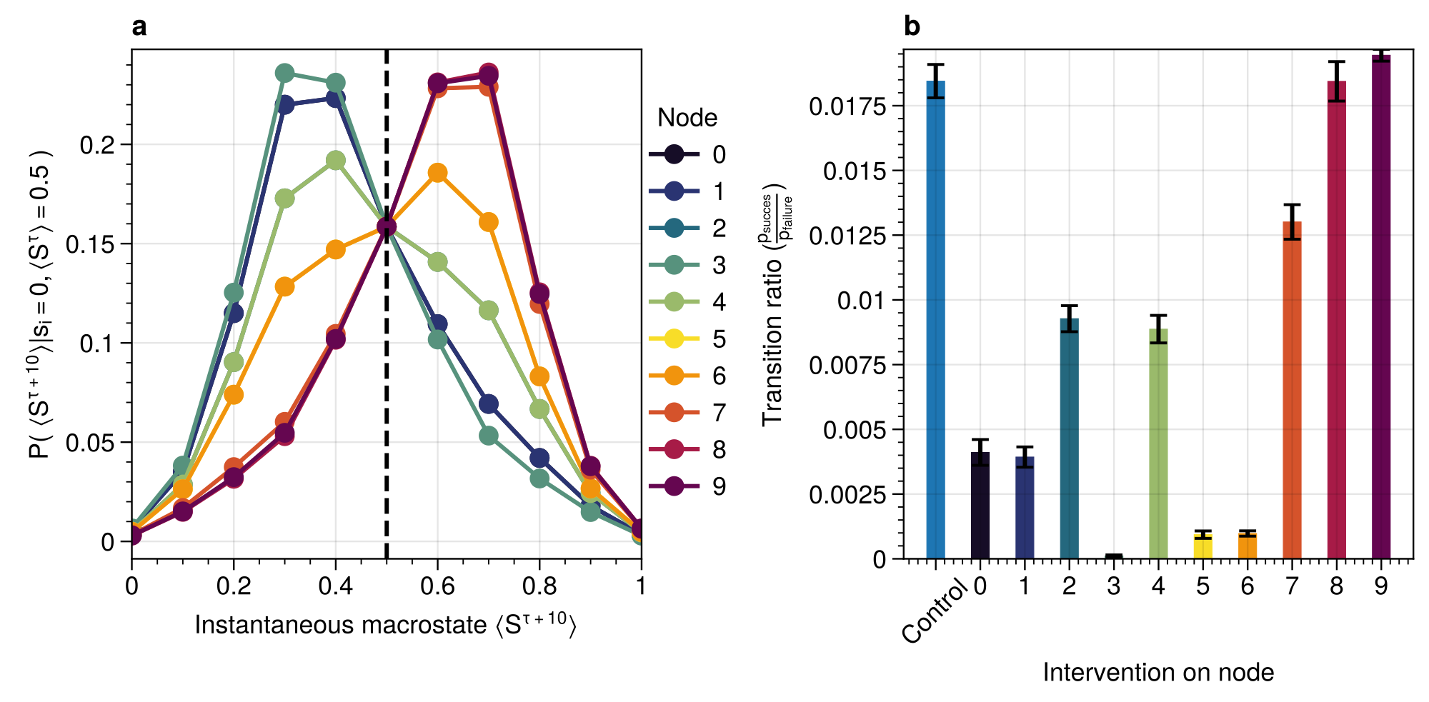
At the tipping point, the system is most likely to either move to a new attractor state or relax back to its original state (Figure 3.3). Path analysis reveals that the most likely paths to the tipping point result in a configuration where a high-degree cluster of nodes must flip. This trajectory is less likely than reversing the path shown in Figure 3.3, explaining why most tipping points “fail” and relax back to the original attractor state (Figure 3.4b).

The increased information of node 8 around the tipping point can be understood by considering its predictive power about the system’s future. As shown in Figure 3.4a, both node 3 and node 8 have low uncertainty about the future system state, but the nature of this certainty differs. Node 3 is more certain that the average system state will equal its state at the tipping point, while node 8 is more certain that the future system state will have the opposite sign to its state at the tipping point.

Role Division and Interventions in Tipping Behavior

We approximate the role of a node $i$ using the difference between integrated mutual information and asymptotic information:

$$\begin{equation} r_i = \max_{\langle S \rangle} \mu^*(s_i | \langle S \rangle) - \max_{\langle S \rangle} \omega^*(s_i) \in [-1, 1], \end{equation}$$

where $\mu^*$ and $\omega^*$ are normalized versions of $\mu$ and $\omega$, respectively.

Nodes with role values close to 1 are classified as “initiators”, with high predictive information about short-lived system trajectories. Nodes with values close to -1 are “stabilizers”, with high long-term predictive information about future system states.

We validated these roles using simulated interventions (Figure 3.5). Pinning initiator nodes to the 0 state promotes tipping points, while pinning stabilizer nodes is essential for stabilizing transitions between attractor states.

Cascades Towards Noise-Induced Transitions on Networks Revealed Using Information Flows

Understanding how metastable transitions occur may help in understanding how, for example, a pandemic occurs, or a system undergoes critical failure. In this chapter, dynamical networks governed by the Boltzmann-Gibbs distribution were used to study how endogenously generated metastable transitions occur. The external noise parameter (temperature) was fixed such that the statistical complexity of the system behavior was maximized (see appendix Section C.II).

The results show that in the network two distinct node types could be identified: initiator and stabilizer nodes. Initiator nodes are essential early in the metastable transition. Due to their high degree of freedom, these nodes are more effected by external noise. They are instigators and propagate noise in the system, destabilizing more stable nodes. In contrast, stabilizer nodes have low degree of freedom and require more energy to change state. These nodes are essential for the metastable behavior as they stabilize the system macrostate. During the metastable transition a domino sequence of node state changes are propagated in an ordered sequence towards the tipping point.

This domino effect was revealed through two information features unveiling an information cascade underpinning the trajectories towards the tipping point.

Integrated mutual information captured how short-lived correlations are passed on from the initiator nodes. In the stable regime (close to the ground state) low degree nodes drive the system dynamics. Low degree nodes destabilize the system, pushing the system closer to the tipping point. In most cases, the initiator nodes will fail in propagating the noise to their neighbors. On rare occasions, however, the cascade is propagated progressively from low degree, to higher and higher degree. A similar domino mechanism was recently found in climate science [112], [115]. Wunderling and colleagues provided a simplified model of the climate system, analyzing how various components contribute to the stability of the climate. They found that interactions generally stabilize the system dynamics. If, however, a metastable transition was initialized, noise was propagated through a similar mechanism as found here. That is, an initializer node propagated noise through the system which created a domino effect that percolated through the system.

An increase in asymptotic information forms an indicator of how close the system is to a tipping point. Close to the ground state, the asymptotic information is low, reflecting how transient noise perturbations are not amplified and the system macrostate relaxes back to the ground state. As the system approaches the tipping point, the asymptotic information increases. As the distance to the ground state increases, the system is more likely to transition between metastable states. After the transition, there remains a longer term correlation. Asymptotic information reflects the long(er) timescale dynamics of the system. This “rest” information peaks at the tipping point, as the system chooses its next state.

The information viewpoint uniquely offers an alternative view to understand how metastable transitions are generated by dynamical networks. Two information features were introduced that decompose the metastable transition in sources of high information processing (integrated mutual information) and distance of the system to the tipping point (asymptotic information). A domino effect was revealed, whereby low degree nodes initiate the tipping point, making it more likely for higher degree nodes to tip. On the tipping point, long-term correlations stabilize the system inside the new metastable state. Importantly, the information perspective allows for estimating integrated mutual information directly from data without knowing the mechanisms that drive the tipping behavior. The results highlight how short-lived correlations are essential to initiate the information cascade for crossing a tipping point.

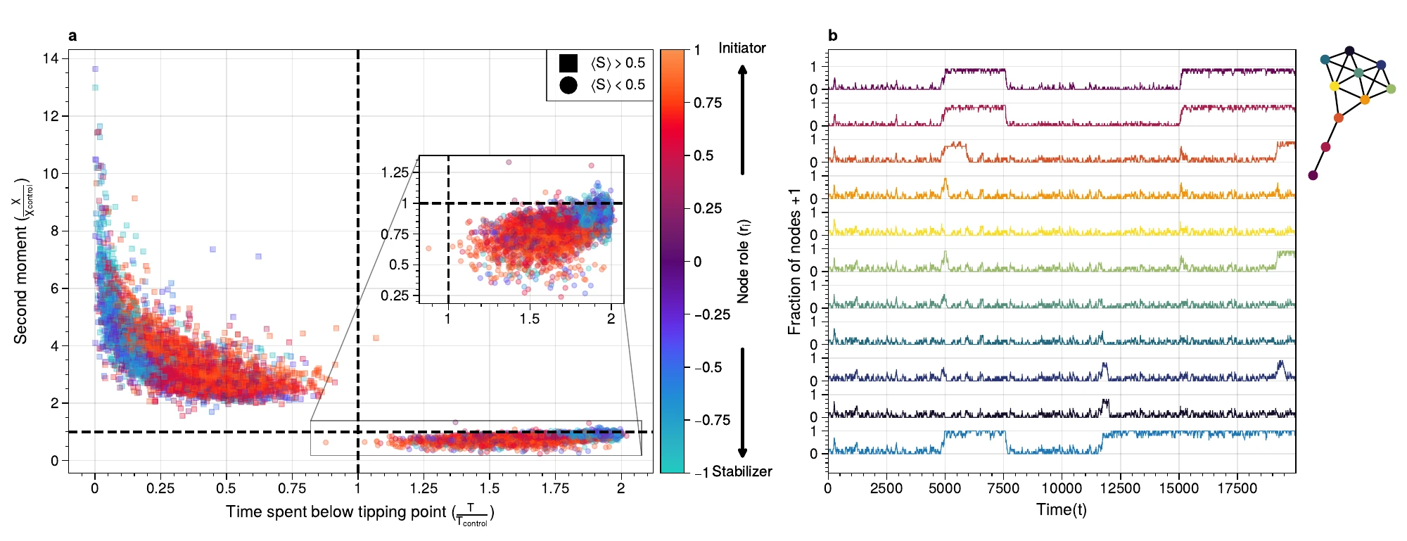
The information theoretic approach offers an alternative view to understand how metastable transitions are generated by dynamical networks. Two information features were introduced that decompose the metastable transition in sources of high information processing (integrated mutual information) and distance of the system to the tipping point (asymptotic information). A domino effect was revealed, whereby low degree nodes initiate the tipping point, making it more likely for higher degree nodes to tip. On the tipping point, long-term correlations stabilizes the system inside the new metastable state. Importantly, the information perspective allows for estimating integrated mutual information directly from data without knowing the mechanisms that drive the tipping behavior. The results highlight how short-lived correlations are essential to initiate the information cascade for crossing a tipping point.