Does Function Imply Form?

Background, scope & innovation

Noise-induced transitions produce metastable behavior that is fundamental for the functioning of complex dynamical systems. For example, in neural systems, the presence of noise enhances information processing through several mechanisms: stochastic resonance, where moderate levels of noise can amplify weak signals and improve signal detection; prevention of neural networks getting stuck in local minima, thereby maintaining system flexibility; and enabling more efficient exploration of different neural states during computation [224], [225], [226], [227]. These effects have been demonstrated both in experimental studies of neural circuits and theoretical models of neural computation.

Similarly, the relation between glacial ice ages and Earth’s eccentricity has been shown to have a strong correlation. Metastability manifests itself through noise that can be of two kinds [97]. External noise originates from events outside the internal system dynamics [98], [228]. Examples include the influence of climate effects, population growth, or random noise sources on transmission lines. External noise is commonly modeled by replacing an external control or order parameter with a stochastic process. Internal noise, in contrast, is inherent to the system itself and is caused by random interactions of elements within the system, e.g., individuals in a population or molecules in chemical processes. Both types of noise can generate transitions between metastable states. In this chapter, we study the metastable behavior of internal noise in complex dynamical networks governed by kinetic Ising dynamics.

The ubiquity of multistability in complex systems calls for a general framework to understand how metastable transitions occur. The diversity of complex systems can be captured by interaction networks that dynamically evolve over time. These dynamics can be seen as a distributive network of computational units, where each unit or element of the interaction network changes its state based on input from its local neighborhood. Lizier demonstrated that the dynamic interaction of complex systems can be understood through their local information processing [64], [229], [230]. Instead of describing the dynamics of the system in terms of domain knowledge such as voltage over distance, disease spreading rate, or climate conditions, one can understand the dynamics in terms of information dynamics. In particular, the field of information dynamics is concerned with describing system behavior through its capacity to store, transmit, and modify information. By abstracting away the domain details of a system and recasting the dynamics in terms of how the system computes its next state, one can capture the intrinsic computations a system performs. The system behavior is encoded in terms of probability, and the relationships among these variables are explored using the language of information theory [74].

Information theory offers profound benefits over traditional methods used in meta-stability analysis, as the methods developed are model-free, can capture non-linear relationships, can be used for both discrete and continuous variables, and can be estimated directly from data [61]. Shannon information measures, such as mutual information and Fisher information, can be used to study how much information the system dynamics shares with the control parameter [99], [231].

Past research on information flows and metastable transitions focuses on methods to detect the onset of a tipping point [232], [233], [234]. It often centers around an observation that the system’s ability to absorb noise reduces prior to the system going through a critical point. This critical slowing down can be captured as a statistical signature where the Fisher information peaks [235]. However, these methods traditionally use some form of control parameter driving the system towards or away from a critical point. Most real-world systems lack such an explicit control parameter and require different methods. Furthermore, detecting a tipping point does not necessarily lead to further understanding of how the tipping point was created. For example, in a finite-size Ising model, the system produces bistable behavior. As one increases the noise parameter, the bistable behavior disappears. The increase in noise effectively changes the energy landscape, but little information is gained about how the metastable behavior initially emerged.

In this work, a novel approach using information theory is explored to study metastable behavior. The statistical coherence between parts of the system is quantified by the capability of individual nodes to predict the future behavior of the system [64]. Two information features are introduced: Integrated mutual information measures predictive information of a node on the future of the system, and Asymptotic information measures the long timescale memory capacity of a node. These measures differ from previous information methods such as transfer entropy [236], conditional mutual information under causal intervention [68], causation entropy [70], and time-delayed variants [237] in that these methods are used to infer the transfer of information between sets of nodes by possibly correcting for a third variable. Here, instead, we aim to understand how the elements in the system contribute to the macroscopic properties of the system. It is important to emphasize that information flows are not directly comparable to causal flows [73]. A rule of thumb is that causal flows focus on micro-level dynamics ($X$ causes $Y$), whereas information flows focus on the predictive aspects, providing a holistic view of emergent structures [64]. In this sense, this work is similar to predictive information [238] where predictive information of some system $(S)$ is projected onto its consistent elements $(s_i \in S)$ and computed as a function of time $(t)$.

Methods and definitions

To study metastable behavior, we consider a system as a collection of random variables $S = \{s_1, \dots, s_n\}$ governed by the Boltzmann-Gibbs distribution:

$$p(S) = \frac{1}{Z} \exp(-\beta \mathcal{H}(S)),$$

where $\beta = \frac{1}{T}$ is the inverse temperature which controls the noise in the system, and $\mathcal{H}(S)$ is the system Hamiltonian which encodes the node-node dynamics. The choice of the energy function dictates what kind of system behavior we observe. Here, we focus on arguably the simplest models that show metastable behavior: the kinetic Ising model and the Susceptible-Infected-Susceptible model.

Temporal dynamics are simulated using Glauber dynamics sampling. In each discrete time step, a spin is randomly chosen and a new state $X'\in S$ is accepted with probability

$$\begin{equation} \begin{split} p(\text{accept } X') = \frac{1}{1 + \exp(-\beta \Delta E)}, \end{split} \end{equation}$$(C.1)

where $\Delta E = \mathcal{H}(X') - \mathcal{H}(X)$ is the energy difference between the current state $X$ and the proposed state $X'$.

Kinetic Ising model

The traditional Ising model, originally developed to study ferromagnetism, is considered one of the simplest models that generate complex behavior. It consists of a set of binary distributed spins $S = \{s_1, \dots, s_n\}$. Each spin contains energy given by the Hamiltonian:

$$\begin{equation} \begin{split} \mathcal{H}(S) = -\sum_{i,j} J_{ij} s_{i} s_{j} - h_{i} s_{i}, \end{split} \end{equation}$$(C.2)

where $J_{ij}$ is the interaction energy of the spins $s_i, s_j$.

The interaction energy effectively encodes the underlying network structure of the system. Different network structures are used in this study to provide a comprehensive numerical overview of the relation between network structure and information flows (see Section C.II). The interaction energy $J_{ij}$ is set to 1 if a connection exists in the network.

For sufficiently low noise (temperature), the Ising model shows metastable behavior (Figure 3.1c). Here, we aim to study how the system goes through a tipping point by tracking the information flow per node with the entire system state.

Information flow on complex networks

Informally, information flows measure the statistical coherence between two random variables $X$ and $Y$ over time, such that the present information in $Y$ cannot be explained by the past of $Y$ but rather by the past of $X$. Estimating information flow is inherently difficult due to the presence of confounding factors, which potentially trap the interpretation in the "correlation does not equal causation" paradigm. Under some contexts, however, information flow can be interpreted as causal [45]. Let $S=\{s_1, \dots, s_n\}$ be a random process, and $S^t$ represent the state of the random process at some time $t$. The information present in $S$ is given as the Shannon entropy:

$$\begin{equation} \begin{split} H(S) = -\sum_{x \in S} p(x) \log p(x), \end{split} \end{equation}$$(C.3)

where $\log$ is base 2 unless otherwise stated, and $p(x)$ is used as shorthand for $p(S = x)$. Shannon entropy captures the uncertainty of a random variable; it can be understood as the number of yes/no questions needed to determine the state of $S$. This measure of uncertainty naturally extends to two variables with Shannon mutual information. Let $s_i$ be an element of the state of $S$, then the Shannon mutual information $I(S; s_i)$ is given as:

$$\begin{equation} \begin{split} I(S; s_i) &= \sum_{S_i\in S, s' \in s_i} p(S_i,s') \log \frac{p(S_i,s')}{p(S_i)p(s')}\\ &= H(S) - H(S | s_i). \end{split} \end{equation}$$(C.4)

Shannon mutual information can be interpreted as the uncertainty reduction of $S$ after knowing the state of $s_i$. Consequently, it encodes how much statistical coherence $s_i$ and $S$ share. Shannon mutual information can be measured over time to encode how much information (in bits) flows from state $s_i^{\tau}$ to $S^{\tau + t}$:

$$\begin{equation} \begin{split} I(S^{\tau + t}; s_i^{\tau}) = H(S^{\tau + t}) - H(S^{\tau + t} | s_i^{\tau}). \end{split} \end{equation}$$(C.5)

Prior results showed that the nodes with the highest causal importance are those nodes that have the highest information flow (i.e., maximize Equation C.5) [45]. Intuitively, the nodes for which the future system "remembers" information from a node in the past are the ones that "drive" the system dynamics. Formally, these driver nodes can be identified by computing the total information flow between $S^t$ and $s_i$, which can be captured with the integrated mutual information [45]:

$$\begin{equation} \begin{split} \mu(s_i) = \sum_{\tau = 0}^{\infty} I(s_{i}^{t-\tau} ; S^t). \end{split} \end{equation}$$(C.6)

In some contexts, the nodes that maximize (C.6) are those nodes that have the highest causal influence in the system [45]. However, in general, information flows are difficult to equate to causal flows [64], [73]. Here, the local information flows are computed by considering the integrated mutual information conditioned on part of the entire state space. This allows for mapping the local information flows between nodes and the system over time but does not guarantee that the measured information flows are directly causal. The main reason is that having predictive power about the future could be completely caused by the partitioning. In [45], the correlation measured considered all possible states, and the measures were directly related to a causal effect.

In addition, in [45], the shared information between the system with a node shifted over time ($I(S^{\tau} : s_i^{\tau + t})$) was considered. Applying this approach under a state partition $I(S^{\tau} : s_i^{\tau + t} | \langle S \rangle)$ causes a violation of the data processing inequality, as information may flow from a node at a particular time $t = t_1$ and then flow back to the node at $t = t_2$, where $t_2 > t_1$. To simplify the interpretation of the information flows and maintain the data processing inequality, the reverse $I(S^{t + \tau} : s_i^{\tau} | \langle S \rangle)$ was computed in the present study.

Noise matching procedure

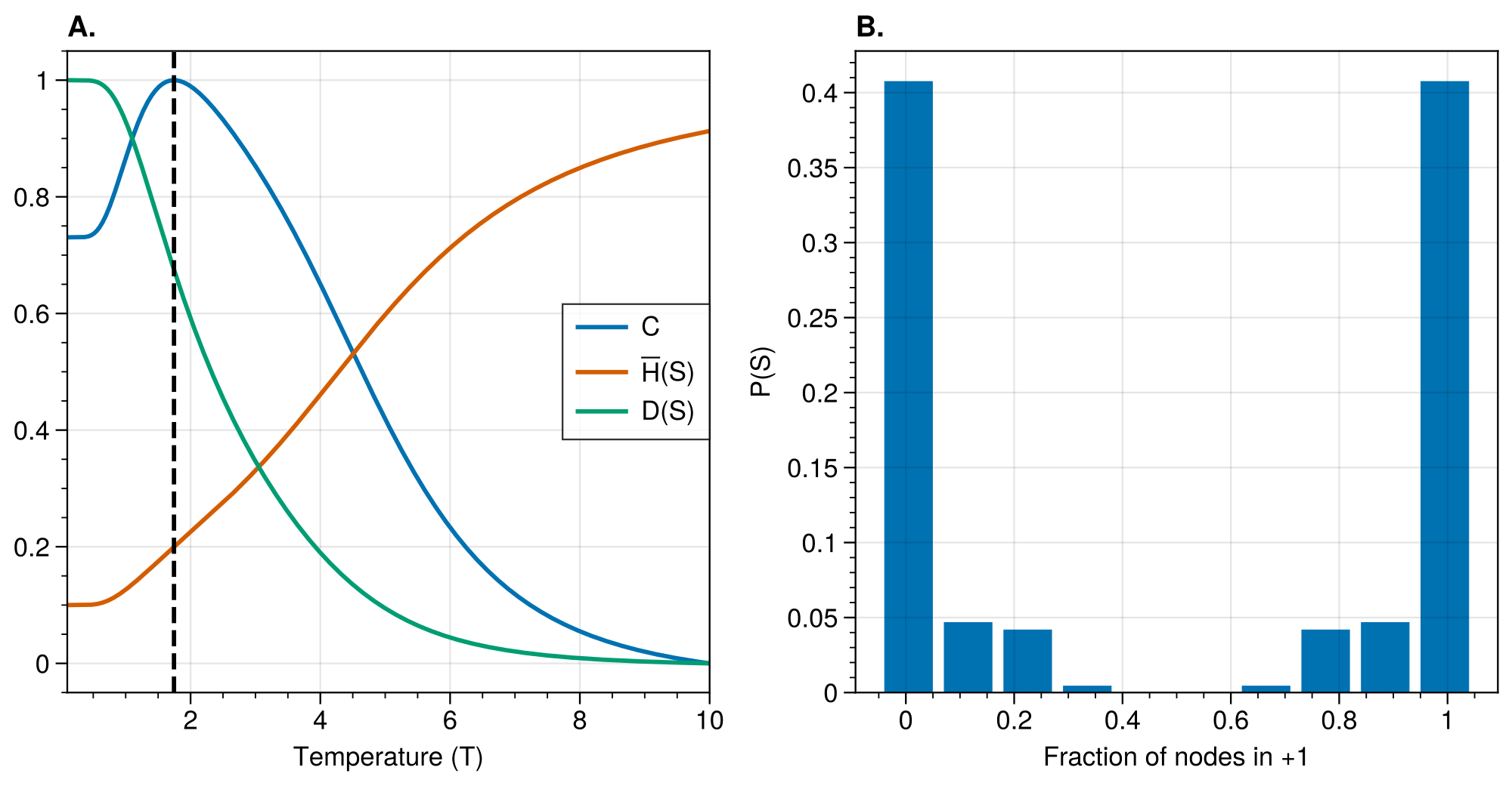
The Boltzmann-Gibbs distribution is parameterized by noise factor $\beta = \frac{1}{kT}$, where $T$ is the temperature and $k$ is the Boltzmann constant. For high $\beta$ values, metastable behavior occurs in the kinetic Ising model. The temperature was chosen such that the statistical complexity [239] was maximized. The statistical complexity $C$ is computed as:

$$C = \bar{H}(S) D(S),$$

where $\bar{H}(S) = \frac{H(s)}{-\log_2(|S|)}$ is the system entropy, and $D(S)$ measures the distance to disequilibrium:

$$D(S) = \sum_i (p(S_i) - \frac{1}{|S|})^2.$$

A typical statistical complexity curve is shown in Figure C.II.1. The noise parameter $\beta$ is set such that it maximizes the statistical complexity using numerical optimization (COBYLA method in scipy’s optimize.minimize module) [240].

Exact information flows $I(s_i^{\tau} ; S^{\tau + t})$

In order to compute $I(s_i^{\tau} : S^{\tau + t})$, the conditional distribution $p(S^{\tau + t} | s_i^{\tau})$ and $p(S^{\tau + t})$ need to be computed. This is achieved through direct computation on the partitions of the state consisting of number of bits flipped – effectively encoding the distance towards or away from a tipping point.

We partition the state space based on the average magnetization $\langle S \rangle$, allowing us to track states that are $n$ bit flips away from the tipping point.

For Glauber dynamics, the system $S$ transitions into $S'$ by randomly choosing node $s_i$ to potentially flip. The transition matrix $p(S^t | s_i) = \textbf{P}$ can be constructed by computing each entry $p_{ij}$ as:

$$\begin{split} p_{ij, i \neq j} &= \frac{1}{|S|} \frac{1}{1 + \exp(-\Delta E)}, \textrm{ with}\\ p_{ii} &= 1 - \sum_{j, j \neq i} p_{ij}, \end{split}$$(C.II.4)

where $\Delta E = \mathcal{H}(S_j) - \mathcal{H}(S_i)$ encodes the energy difference of moving from $S_i$ to $S_j$.

For each partition $S_{\gamma} = \{S' \subseteq S | \langle S' \rangle = \gamma\}$, we:

1. Compute transition probabilities between states within the partition

2. Renormalize probabilities to ensure conservation within the partition

3. Evaluate $p(S^t | s_i)$ for all possible node states $s_i$ in that partition

The marginal distribution $p(S^t)$ is then computed as:

$$p(S^{\tau + t}) = \sum_{s_i} p(S^{\tau + t} | s_i^{\tau}) p(s_i^{\tau}).$$

This procedure provides exact information flows for states at specific distances from the tipping point, allowing us to track how correlations evolve as the system approaches and moves away from the transition.

Extrapolation with regressions

Exact information flows were computed per graph for $t = 500$ time steps. Using ordinary least squares, a double exponential was fit to estimate the information flows for longer $t$ and estimate the integrated mutual information and asymptotic information.

Noise estimation procedure

Tipping point behavior under intervention was quantified by evaluating the level of noise on both sides of the tipping point. Let $T_1$ represent the ground state where all spins are 0, $T_2$ where all spins are 1, and let the tipping point $TP$ be where the instantaneous macrostate $M(S^t) = 0.5$. Fluctuations of the system macrostate were evaluated by analyzing the second moment above and below the tipping point. This was achieved by numerically simulating the system trajectories under 6 different seeds for $t = 10^6$ time steps. The data was split between two sets (above and below the tipping point), and the noise $\eta$ was computed as:

$$\begin{equation*} \begin{split} \eta = \frac{1}{\alpha^2 |S_{w}|} \sum_w {S_w^t}^2, \end{split} \end{equation*}$$(C.II.5)

where $w \in \{\langle S \rangle < 0.5, \langle S \rangle > 0.5\}$, and

$$\begin{equation} S_{w}^{t} = \begin{cases} S^t & \textrm{if } S^t < 0.5 \\ 1 - S^t & \textrm{if } S^t > 0.5 \end{cases} \end{equation}$$(C.7)

is the instantaneous system trajectory for the system macrostate above or below the tipping point value. The factor $\alpha$ corrects for the reduced range the system macrostate has under interventions. For example, pinning a node $s_i$ to state 0 reduces the maximum possible macrostate to $1 - \frac{1}{n}$, where $n$ is the size of the system. The correction factor $\alpha$ is set such that for an intervention on 0 for a particular node, the range $S_{\langle S \rangle > 0.5}$, $\alpha$ is set to $\frac{n}{2} - \frac{1}{n}$.

Switch susceptibility as a function of degree

First, we investigate the susceptibility of a spin as a function of its degree. The susceptibility of a spin switching its state is a function of both the system temperature $T$ and the system dynamics. The system dynamics contribute to the susceptibility through the underlying network structure either directly or indirectly. The network structure produces local correlations which affect the switch probability for a given spin.

As an initial approximation, we consider the susceptibility of a target spin $s_i$ to flip from a majority state to a minority state given the state of its neighbors, where the neighbors are not connected among themselves. Further, we assume that for the instantaneous update of $s_i$, the configuration of the neighborhood of $s_i$ can be considered as the outcome of a binomial trial. Let $N$ be a random variable with state space $\{0, 1\}^{|N|}$, and let $n_j \in N$ represent a neighbor of $s_i$. We assume that all neighbors of $s_i$ are i.i.d. distributed given the instantaneous system magnetization:

$$M(S^t) = \frac{1}{|S^t|} \sum_i s_i^t.$$

Let the minority state be 1 and the majority state be 0. The expectation of $s_i$ flipping from the majority state to the minority state is given as:

$$\begin{align*} E[p(s_i = 1 | N)]_{p(N)} = \sum_{N_i \in N} p(N_i) p(s_i = 1 | N_i)\\ = \sum_{N_i \in N} \prod_j^{|N_i|} p(n_j) p(s_i = 1 |N_i)\\ = \sum_{N_i \in N} {n\choose k} f^k (1 - f)^{n-k} p(s_i = 1 | f), \end{align*}$$(C.8)

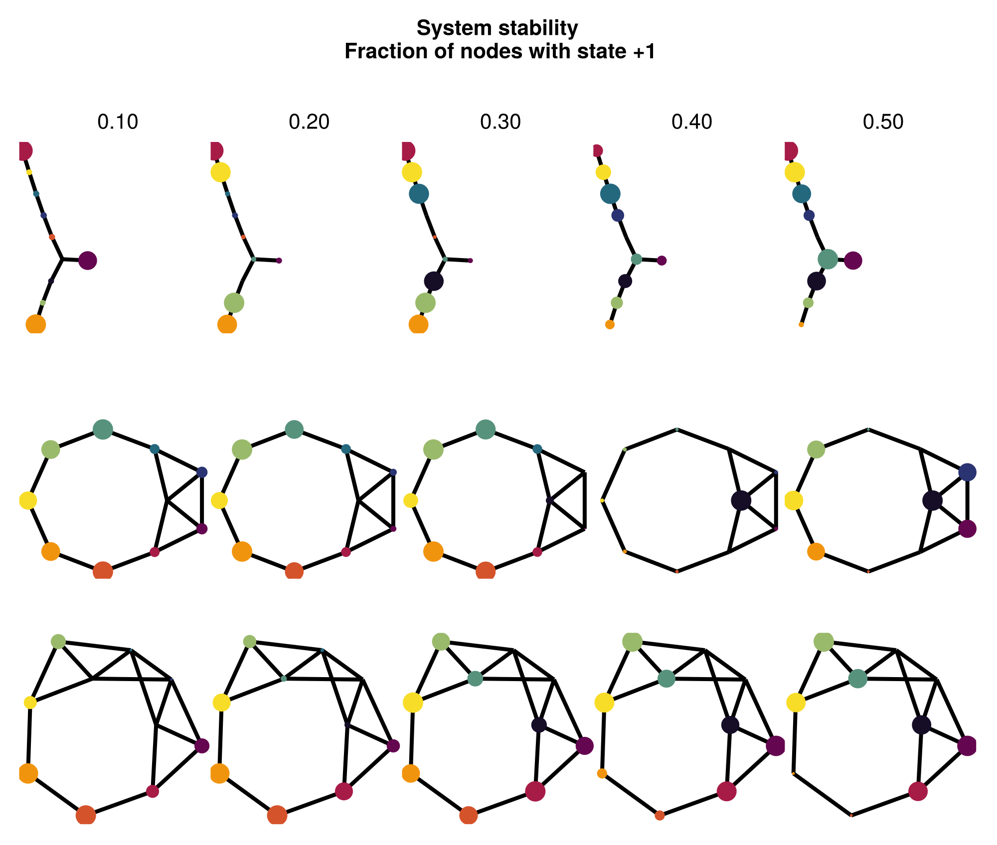
where $f$ is the fraction of nodes in the majority states, $n$ is the number of neighbors, and $k$ is the number of nodes in state 0. As shown in Figure C.V.1, this is computed as a function of the degree of spin $s_i$. As the degree increases, the susceptibility for a spin decreases relative to the same spin with a lower degree. This implies that the susceptibility to change due to random fluctuations is more likely to occur in nodes with fewer external constraints as measured by degree.

Additional networks

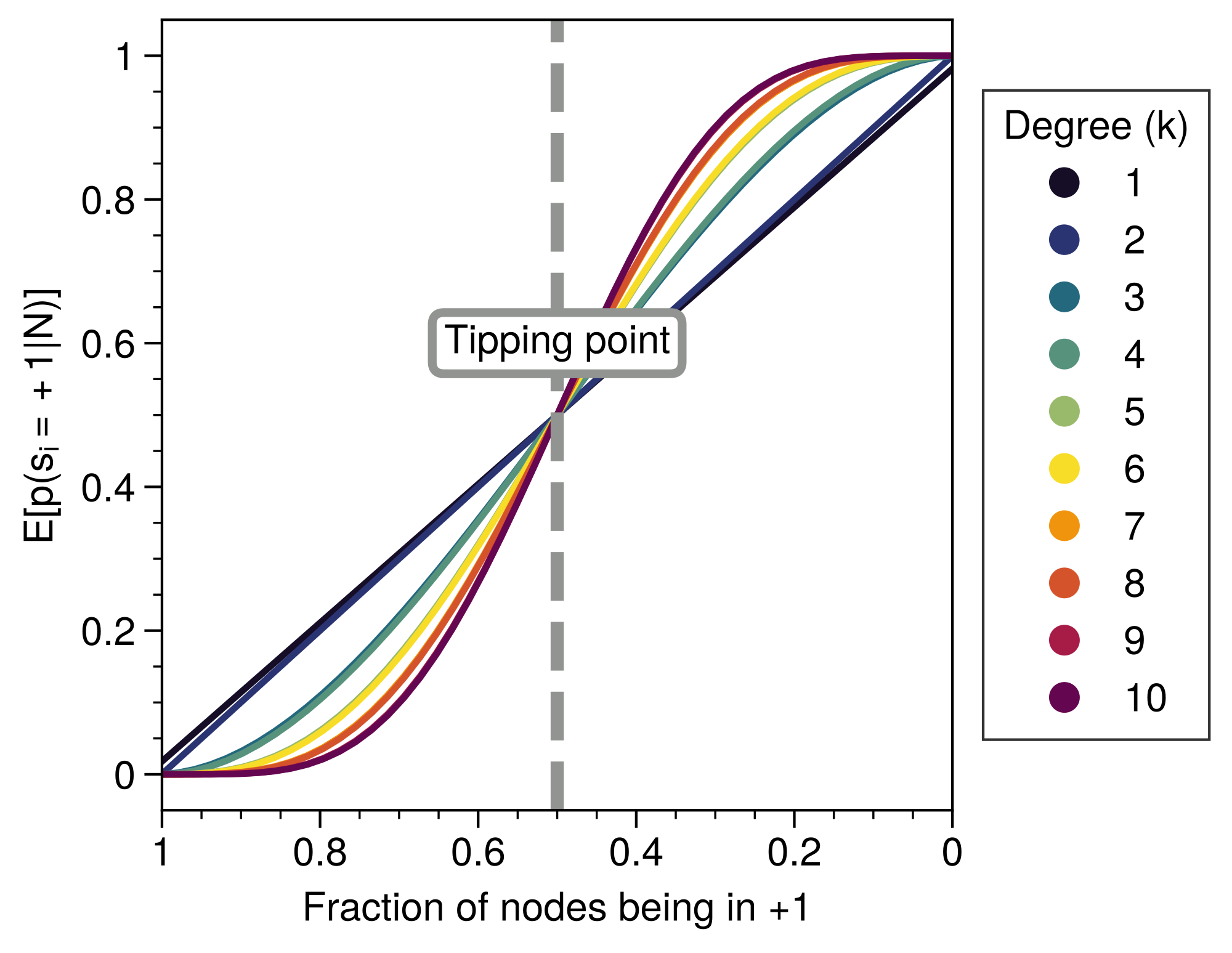
The kite graph was chosen as it allowed for computing exact information flows while retaining a high variety of degree distribution given the small size. Other networks were also tested. In Figure C.IV.1, different network structures were used. Each node is governed by kinetic Ising spin dynamics.

Flip probability per degree

In Figure C.V.1, the tendency for a node to flip from the majority to the minority state is computed as a function of the fraction of nodes possessing the majority state 1 in the system, denoted as $N$. Two things are observed. First, nodes with lower degree are more susceptible to noise than nodes with higher degree. For a given system stability, nodes with lower degree tend to have a higher tendency to flip. This holds true for all distances of the system from the tipping point. In contrast, the higher the degree of the node, the closer the system must be to a tipping point for the node to change its state. This can be explained by the fact that lower-degree nodes have fewer constraints compared to nodes with higher degree. For Ising spin kinetics, the nodes with higher degree tend to be more "frozen" in their node dynamics than nodes with lower degree. Second, for a node to flip with similar probability mass (i.e., $E[p(s_i) | N] = 0.2$), a node with higher degree needs to be closer to the tipping point than nodes with lower degree. In fact, the order of susceptibility is correlated with the degree; the susceptibility decreases with increasing degree and fixed fraction of nodes in state 1.

Synthetic networks

For the synthetic graphs, 100 non-isomorphic connected Erdős-Rényi networks were generated with p = 0.2. Graphs were generated randomly and rejected if they did not contain a giant component or were isomorphic with already generated graphs. For each of the graphs, information curves were computed as a function of the macrostate $\langle S \rangle$.

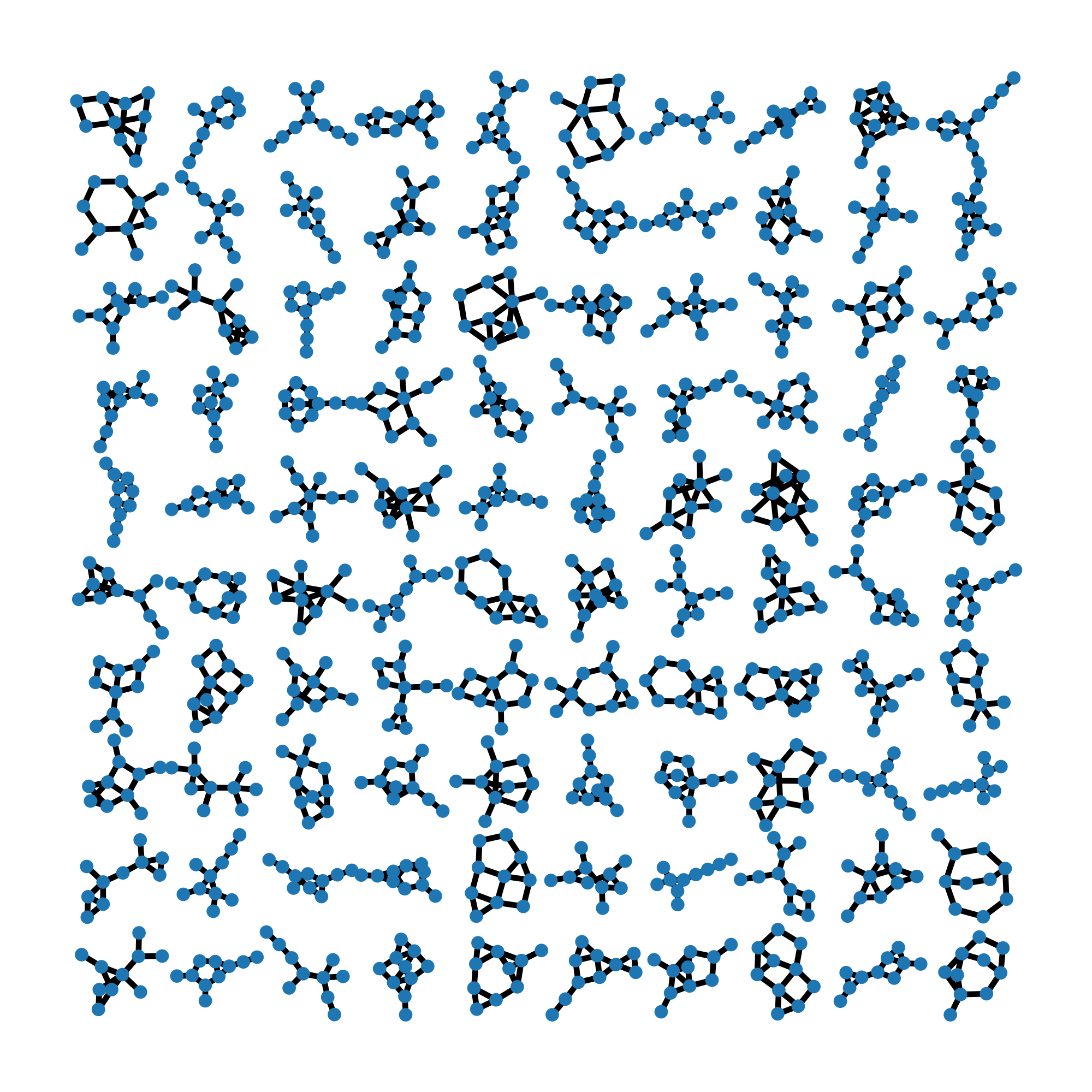
Analysis of Network Variability and Temporal Behavior

Various network structures are generated in the synthetic networks. The variety of network structure has non-linear effects on the information flows. The effect of intervention in Figure 3.5 is made relative to the control values for the graph and seed. The second moment (appendix: Section C.II.5) and the time spent below the tipping point are normalized with respect to the graph (Figure C.VI.1) and the seed. In total, 6 seeds are used (0, 12, 123, 1234, 123456, 1234567).

Case Study of a Larger System

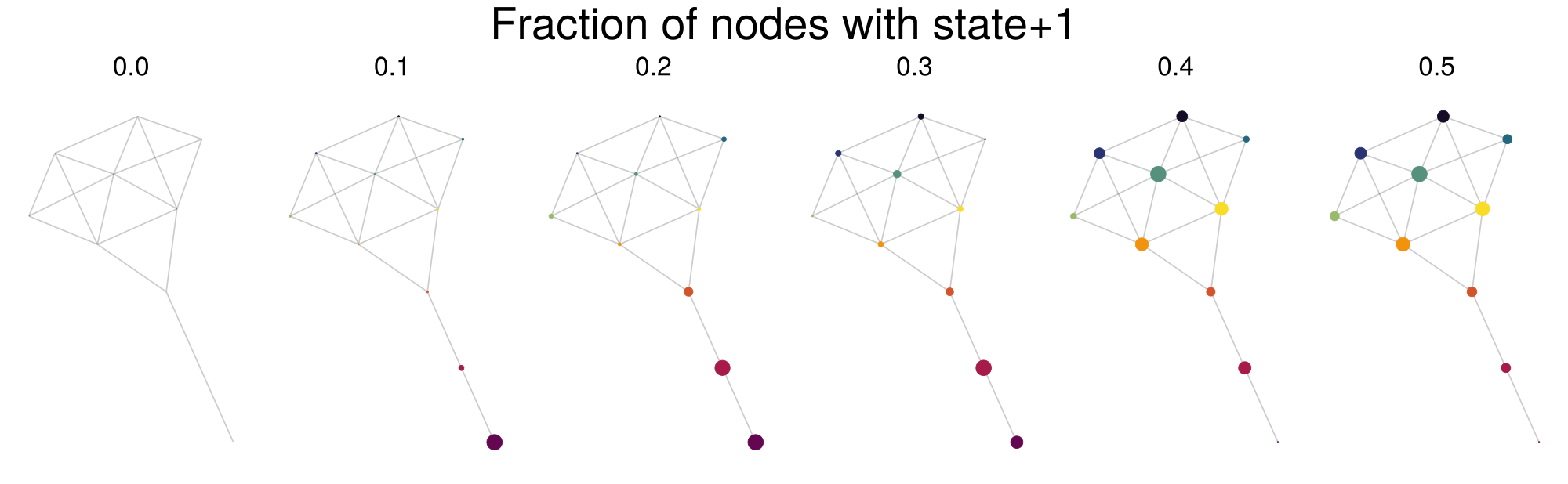
In this section, we extend the analysis to a 15-node network to demonstrate the applicability of the findings to larger systems (see Figure C.VIII.1). This case study serves to validate the theoretical insights derived from smaller networks and to illustrate how the fundamental mechanisms of metastable transitions are preserved as network size increases. Despite the increased computational complexity, the results indicate that the structural features driving these transitions in smaller networks are also evident in larger ones.

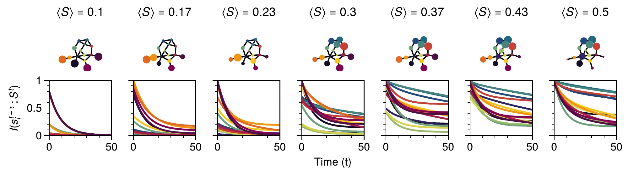
As highlighted in Section C.IX, the state space of a network grows exponentially ($2^n$) with the number of nodes, making simulations of larger systems computationally demanding. Nevertheless, the analysis of the 15-node network supports the assertion that the foundational processes identified in the primary study can be extrapolated to more complex networks. Detailed results and discussion of this 15-node network analysis are provided to substantiate the approach and highlight the consistency of the findings across different network sizes.

Limitations

Integrated mutual information was computed based on exact information flows. This means that for binary systems it requires to compute a transfer matrix on the order of $2^{|S|} \times 2^{|S|}$. This reduced the present analysis to smaller graphs. It would be possible to use Monte-Carlo methods to estimate the information flows. However, $I(s_i^{\tau} : S^{\tau + t})$ remains expensive to compute. When using computational models, it requires to compute the conditional and marginal distributions which are on order $\mathbb{O}(2^{|S|})$ and $\mathbb{O}(2^{t|S|})$ respectively. In Section C.VIII, we give a proof of principle how the results presented here would generalize to larger systems.

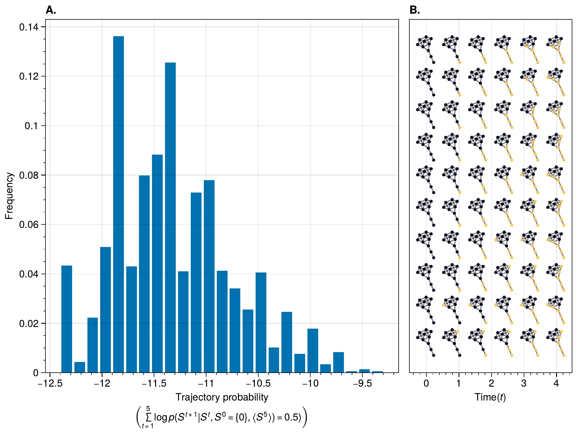
In addition, the decomposition of the metastable transition depends on the partition of the state space. Information flows are in essence statistical dependencies among random variables. Here, the effect of how the tipping point was reached was studied by partition the average system state in terms of number of bits flipped. This partitioning assumes that the majority of states prior to the tipping point are reached by having fraction $c \in [0, 1]$ bits flipped. The contribution of each system state over time, however, reflects a distribution of different states; reaching the tipping point from the ground state 0, can be done at $t-2$ prior to tipping by either remaining in 0.4 bits, or transitioning from 0.3 bits flipped to 0.4 and eventually to 0.5 in 2 time steps. The effect of these additional paths showed marginal effects on the integrated mutual information and asymptotic information.

Information flows conditioned on a partition is a form of conditional mutual information [73]. Prior results showed that conditional information produces synergy, i.e. information that is only present in the joint of all variables but cannot be found in any of the subset of each variable. Unfortunately, there is no generally agreed upon definition on how to measure synergy [241], [242] and different estimates exist that may over or underestimate the synergetic effects. By partitioning one can create synergy as for a given partition each spin has some additional information about the other spins. For example, by taking the states such that $\langle S \rangle = 0.1$, each spin “knows” that the average of the system equals 0.1. This creates shared information among the spins. Analyses were performed to estimate synergy using the redundancy estimation $I_{min}$[243]. Using this approach, no synergy was measured that affected the outcome of this study. However, it should be emphasized that synergetic effects may influence the causal interpretation of the approach presented here.

A general class of systems was studied governed by the Boltzmann-Gibbs distribution. For practical purposes the kinetic Ising model was only tested, but we speculate that the results should hold (in principle) for other systems dictated by the Boltzmann-Gibbs distribution. We leave the extension to other system Hamiltonians for future work.

The practical implementation of interventions based on the theoretical framework faces several real-world challenges. First, in actual complex systems, measuring and monitoring the complete state space in real-time may be technically infeasible or prohibitively expensive. Second, the ability to perform precise, targeted interventions on specific components of the system may be limited by physical constraints or technological capabilities. Third, the assumption of perfect knowledge about system parameters and state transitions may not hold in real-world scenarios where noise, measurement errors, and external perturbations are present. Furthermore, the time scales at which interventions need to be implemented may be too rapid for practical human or automated response systems. These practical limitations suggest that while the framework provides valuable theoretical insights, its application may require significant adaptation and simplification for real-world implementation, potentially trading off optimal control for practical feasibility.