Does form imply function?

Understanding dynamical systems is a fundamental problem of the 21st century [46]. This chapter explores the relationship between the structure of a system (form) and its dynamic behavior (function). Despite the apparent differences in various real-world networked complex systems, previous research shows several universal characteristics in network properties such as the small-world phenomenon [47], fat-tail degree distributions [48], and feedback loops [49]. This has led to the common but often implicit assumption that a node’s connectedness in the network is proportional to its dynamic importance [50]. For example, in epidemic research, high-degree nodes or “super-spreaders” are associated with dominant epidemic risk and therefore deserve special attention [51].

Yet, prior research indicates that shared network characteristics do not necessarily translate to shared dynamic or functional properties in these networks [3], [6]. Specifically, a node’s dynamic importance varies depending on both the network dynamics and its structural connectedness. This effect was rigorously demonstrated by Harush and colleagues [3], who varied dynamic processes while keeping network structures constant. They studied both randomly generated and real-world networks, computing nodal importance based on the “information flow" through a node. This flow had a non-linear relationship with structural connectedness and the type of dynamics present in the system. These results highlight the complex interplay between a system’s structure and the dynamics between its nodes.

However, the results required full knowledge of the system, meaning both the network structure and dynamics were necessary to estimate the node with the highest dynamic importance. For real-world systems, having both dynamics and underlying network structure available can be challenging. Additionally, their study assumed a constant network structure, leaving it unclear whether the proposed flow would generalize to systems with varying structures. The results were also obtained from steady-state analyses. For dynamical processes, an out-of-equilibrium approach can highlight how trajectories generate systemic behavior. What is needed are methods to detect the highest dynamic importance of a node from observations directly, without knowing or assuming the underlying network or causal structure among variables.

Traditionally, a node’s dynamic (or causal) importance is inferred through interventions and counterfactuals [52], [53]. External interventions can change system behavior, with high causal importance relating to significant changes in system behavior. Studies using causal interventions often apply “hard” intervention strategies [54], where a node is pinned to a state, effectively removing all incoming connections and influences from the system. This approach is common in various disciplines, such as gene-knockout experiments, epidemic spreading, network analysis, and driver node identification.

Identifying nodes with high dynamical importance, referred to as driver nodes, through external interventions is challenging for three reasons. First, hard interventions may cause systemic behavior changes that do not occur in non-intervened behavior or may be impractical (e.g., requiring infinite resources) [55]. This complicates theory formation regarding the mechanisms underlying observed systemic behavior. Second, most causal inference approaches assume causal interactions follow a particular structure without local loops [56], [57], [58]. This assumption simplifies theoretical analysis but presumes the underlying causal structure is known or accessible. If not known, it must be inferred from data, which poses challenges in terms of temporal resolution and scale. Real-world systems often have cyclical causal structures, making it difficult to determine the correct temporal scale for causal interactions. Third, the underlying causal structure may be unknown or difficult to determine [59]. Many dynamical systems prohibit analytical approaches to directly decompose each node’s dynamical importance due to polyadic, often non-linear interactions [1].

For closed systems, it is possible to deduce the driver node by considering cross-sectional time series and computing the correlation of each node with the entire system out-of-equilibrium without lossy compression [60]. Here, a driver node is the element most correlated with the entire system over time, having the maximum dynamic (causal) impact when intervened upon. By considering the entire system, internal confounding information is implicitly accounted for, excluding any other node from having more dynamic importance than the node with the highest correlation.

Shannon information theory offers significant advantages over previous approaches for defining a measure of the dynamical importance of a driver node on the behavior of all other nodes [61]. Firstly, Shannon mutual information can quantify statistical associations among variables without bias to specific forms of association [62]. It equals zero if the full probability distribution of the system state remains unchanged regardless of the node’s state. Secondly, mutual information does not require prior knowledge of the system’s representational base, allowing direct comparison among different systems with various units of measurement. Finally, it is defined for both discrete-valued and real-valued state variables.

Measuring the dynamic importance of a node through information flow is not new. Information flows from process $X$ to process $Y$ represent statistical coherence between the present information in $Y$ and the past of $X$ not accounted for by the past of $Y$. Various methods, such as transfer entropy [63] and its derivatives [64], [65], [66], [67], extend the notion of information flow to causal influence or dynamic importance. Previous research developed measures for determining how much information flow between two processes is truly causal, such as conditional mutual information under causal intervention [68], causation entropy [69], permutation conditional mutual information [70], and time-delayed Shannon mutual information [71].

These measures infer information transfer between nodes by possibly correcting for a third confounding variable [54], [72]. However, in polyadic settings, most measures of information flow can underestimate or overestimate nodal importance [73]. Determining how much information flow is causal between source and sink variables in polyadic settings is difficult due to synergetic and redundant information [73], [74].

Instead of focusing on the open problem of full information decomposition among variables, we focus on the amount of information that a node shares with the entire system. A driver node is expected to have a high information flow from it to the system. we introduce a novel metric named integrated mutual information (IMI) based on time-delayed Shannon mutual information with a node and the entire system over time, capturing driver nodes with the highest causal impact in ergodic systems. By avoiding conditional mutual information, we sidestep confounding information synergy with redundancy. We quantify only how much causal impact one single node has on the entire network, without inferring which parts of the network are impacted more or how the causal influence percolates. This is sufficient for this study’s purpose.

Using this approach, it was previously shown analytically that the number of connections of a node does not necessarily scale monotonically with its dynamical importance in infinite-sized, locally-tree-like networks (i.e., networks without loops) [75]. For these networks, nodes with high dynamic importance were not necessarily the high-degree nodes (hubs). Instead, nodes with intermediate connectedness were identified as having the highest dynamical importance. This study extends prior research by numerically computing information flow in finite-sized, random networks where small feedback loops cannot be ignored, and examines the relationship between connectivity and dynamic importance of nodes in such networks.

The aim of this chapter is to test the common hypothesis that a node’s connectedness is proportional to its dynamical importance. A node’s dynamic importance is determined by simulating the (out-of-equilibrium) dynamics of a system under causal external interventions. The distance between system state probability distributions with and without the intervention is used as a ground truth for a node’s causal influence over time (see Section 2.1.2). The resulting causal impact score is compared with common network centrality metrics (Section B.VI) and our proposed information-based metric.

Unlike other studies, the proposed metrics in this study (Section 2.1) do not assume a specific network structure or type of dynamics. We use small networks (up to 12 nodes) to investigate “network motifs” embedded within larger network structures [76]. By understanding causal flows in these smaller structures, we can gain insights into larger systems composed of smaller network components. Additionally, the smaller network sizes provide a numerical advantage for accurately estimating causal and information measures.

First, we perform a proof of principle on synthetic networks to demonstrate how information can be used to determine dynamic importance comprehensively. The chapter concludes by applying the network to real-world psychological symptom networks. Finally, we discuss the results and their implications within the broader scientific literature.

Bridging Form and Function through Discrete-Time Dynamics

Terminology and Definitions

In this chapter, we consider a complex system as a set of discrete random variables $S = \{s_1, s_2, \dots, s_n\}$ with interaction structure $E = \{(s_i, s_k) | s_i, s_k \in S\}$, where each $s_i \in S$ has an alphabet $A$. This is also known as a (discrete) dynamical network [77]. Please note that we use the term node and variable interchangeably referring to an element $s_i \in S$. The system chooses its next state $S^t$ in discrete time with probability:

$$\begin{equation} \begin{split} p(S^t | S^{t-1}, \dots, S^{t_0}) = p(S^{t} | S^{t-1}), \end{split} \end{equation}$$

which is also known as a first-order Markov chain. More specifically, each discrete time step, a single variable $s_i \in S$ is chosen with uniform probability and updated. That is,

$$\begin{equation} \begin{split} p(S^t | S^{t-1}, \dots, S^{t_0}) = p(S^{t} | S^{t-1}) = \prod_j p(s_j^{t} | S^{t-1}) = p(s_i^{t} | S^{t-1}). \end{split} \end{equation}$$(2.2)

For temporal dynamics, we adopt here the Metropolis-Hasting algorithm [78]. By drawing a proposal state $S^{t+1} = X'$ from current state $S^t = X$ from a proposal distribution $g(X' | X)$ and accepting the new state $X'$ with probability,

$$\begin{equation} \begin{split} A(S^{t+1} = X', S^t = X) &= \min\big(1, \frac{p(S^{t+1} = X') g(S^{t+1} = X | S^t = X')}{p(S^t = X) g(S^{t + 1} = X' | S^t = X)}\big)\\ &= \min\big(1, \frac{p(s_i^{t+1} = x') g(s_i^{t} = x | s_i^{t} = x')}{p(s_i^{t+1} = x) g(s_i^{t} = x' | s_i^{t} = x)}\big), \end{split} \end{equation}$$ where $x' \in A$. If the new state is not accepted, then the next state will be set to $S^{t+1} = X$. As the next state $S^{t+1}$ is determined through considering updating a single variable $s_i \in S$, the next state $X'$ will be generated through the proposal state $x'$ drawn uniformly from the possible states $A$ such that $g(x' | x) = g(x | x') = g(x') = \frac{1}{|A|}$. This means that $\frac{g(X' | X)}{g(X | X')} = \frac{g(x' | x)}{g(x | x')} = 1$.

For our experiments, we use the kinetic Ising model which is thought to fall in the same universality class as various other complex behaviors [39], such as (directed) percolation, diffusion, and many extensions of the model have been used as a base for opinion dynamics, modeling neural behavior and so on. For demonstrating our primary claim that high network connectivity does not necessarily lead to high dynamical importance, a single dynamics suffices as counterexample.

It is nevertheless important to emphasize that our proposed driver node inference method does not depend on the exact type of dynamics. That is, the choice for the kinetic Ising spin dynamics is arbitrary in that respect. Our methods only require that for a given dynamics the data-processing inequality is satisfied. More details on the methods and its assumption will follow in Section 2.1.3.

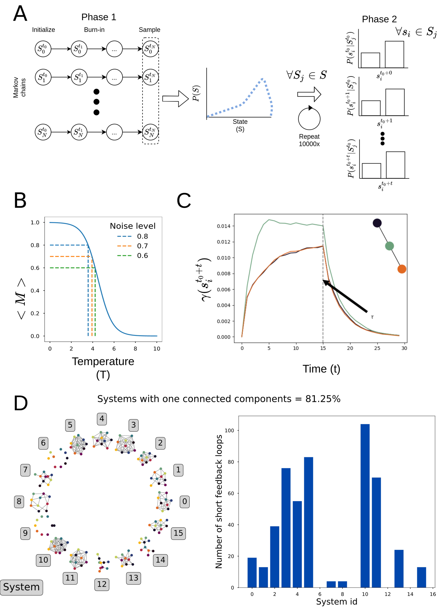
The kinetic Ising model consists of binary variables dictated by a Gibbs distribution that interact through nearest neighbor interactions. A prominent property of the Ising model in higher dimensions (two or more) is the phase transition from an ordered phase to a disordered phase by increasing the noise parameter $\beta$. For finite systems, the kinetic Ising model shows a continuous phase transition from ordered to unordered system regime ( Figure 2.4 B). The Metropolis-Hastings update rule specifically for the kinetic Ising model equals:

$$\begin{equation} \begin{split} p( \text{accept } X' ) = \frac{p(X')}{p(X)} = \begin{cases} 1 & \text{if } \mathcal{H}(X') - \mathcal{H}(X) < 0\\ \exp(-\beta (\mathcal{H}(X') - \mathcal{H}(X)) & \text{otherwise,} \end{cases} \end{split} \end{equation}$$(2.4)

where $\mathcal{H}(S)$ is the system Hamiltonian defined as

$$\begin{equation} \begin{split} \mathcal{H}(S) = -\sum_{i,j} J_{ij} s_{i} s_{j} - h_{i} s_{i}. \end{split} \end{equation}$$(C.2)

Here $\beta$ is the inverse temperature $\frac{1}{k_b T}$ with Boltzmann constant $k_b$, $J_{ij}$ is the interaction strength between variables $s_i$ and $s_j$; $h_i$ represents external influence on node $i$. The matrix $J$ effectively represents the network of the system: an edge between $s_i, s_j \in S$ exists if $|J_{ij}| > 0$. The networks considered in this study are undirected networks, which means that $J$ is an $|S| \times |S|$ symmetric matrix. For the randomly generated networks the edges $J_{ij} \in \{0, 1\}$; for the real network dataset the edge weights are positive and negative real numbers (section 2.2).

The $\beta$ parameter can be seen as the (inverse) noise parameter in the system. Low values of $\beta$ will induce each node in the system to detach from the influence of its neighbors, i.e. the probability of finding a node in a state $p(s_i = a), a \in A$ will tend to uniform distribution as $\beta \rightarrow 0$. In contrast, high values of $\beta$ increases the influence a neighbor of a node may have on determining the node’s next state.

Dynamic Importance Inferred Through Causal Interventions

We call a node a driver node for a dynamical system when it has the largest causal impact on the system dynamics. In brief, we will determine a node’s causal impact by simulating a transient intervention and subsequently quantifying the difference between the system dynamics under intervention and without intervention. We expect that the impact of the driver nodes will penetrate deeper into the system and remain present longer than for nodes with lower causal impact. Here, we define causal impact by means of external intervention on a node. The external causal intervention $\vec{\epsilon}$ on node $s_j \in S$ can be described as

$$\begin{equation} \begin{split} p_{s_j}'(s_i^t | S^{t-1}) = p(s_i^t | S^{t-1}) + \vec{\epsilon}\delta_{ij}, \end{split} \end{equation}$$(2.6)

where $\delta_{ij}$ is the Kronecker-delta, and $\textrm{dim}(\vec{\epsilon}) = |A|$. In addition, $\sum_{i = 0}^{|A|} \epsilon_i = 0$ and $\sum_{i = 0}^{|A|} |\epsilon_{i}| = c$ for some $c \in (0, 1]$. Note only those $\vec{\epsilon}$ are allowed that generate valid new probabilities, i.e. $0 \leq p' \leq 1$.

Relative to some equilibrium distribution $p(S^{\tau})$, the effect of intervention $\vec{\epsilon}$ will result in a new system state equilibrium distribution $p'(S^{\tau})$. Subsequently the intervention is removed at a random system state, after which the distribution of system states will gradually converge back to the original equilibrium. Nodes with higher dynamic importance will cause a larger difference in the system state probability distribution over time. Consequently, we quantify the causal impact of a node by integrating over time $t$ the difference in system state distribution from the moment the intervention is released ($t = \tau$). Since our model is discrete in time, the integral becomes a summation. Thus, we define the causal impact of node $s_i \in S$ as

$$\begin{equation} \begin{split} \Gamma(s_i) &= \sum^\infty_{t= \tau} \gamma(s_i^{t }) \Delta t\\ &= \sum_{t = \tau}^\infty \sum_{s_j \in S} D_{KL}(p'_{s_i}(s_j^{t}) || p(s_j^{t}) ) \Delta t \end{split} \end{equation}$$(2.7)

where $D_{KL}$ is the KL-divergence, and $\Delta t = 1$ throughout the chapter. KL-divergence $D_{KL}(p || q)$ quantifies the difference between probability distributions and is non-negative, invariant under affine parameter transformation and zero when $p = q$. For example, if $\Gamma(s_i) = 0$ the intervention on nodes $i$ caused no difference in any state probabilities.

The driver node can then readily be defined as $\textrm{argmax}_{s_i \in S}(\Gamma(s_i))$. A numerical implementation of driver node identification is given in Section 2.2.2.

In this study, we allow the intervention to evolve for some time period $\Delta t_{\textrm{nudge}} = \tau - t_0$ after which the nudge is removed (see Section 2.2.2 and Figure 2.4 C). The intervention will transiently bring the system out of equilibrium. For ergodic systems, the effect of the intervention will be lost from the system over time. Namely, $P_{s_i}'(S), \forall s_i$ will tend to equilibrium distribution $P(S)$ from $\tau$ on wards. The causal impact is computed relative to this $\tau$ (Figure 2.4 C). As a consequence $\Gamma(s_i)$ will be finite for systems under study here, but may diverge for non-ergodic systems. The duration $\tau$ needs to be set appropriately that the intervention is allowed to percolate through the system. Here we used $\tau = 15$ for random networks consisting of 10 nodes and $\tau = 25$ for the real-world weighted network consisting of 12 nodes (see Section 2.2.1).

The time prior to $\tau$ is used for computing the causal impact on a node as the intervention could be disproportional affected by the act of changing the node distribution. It does not accurately reflect the causal impact of the node on the rest of the system. Only the decay after $\tau$ would be proportional to the causal impact a node has on all other nodes. The causal impact is therefore computed based on the decay of the causal impact relative to $\tau$.

Intervention size

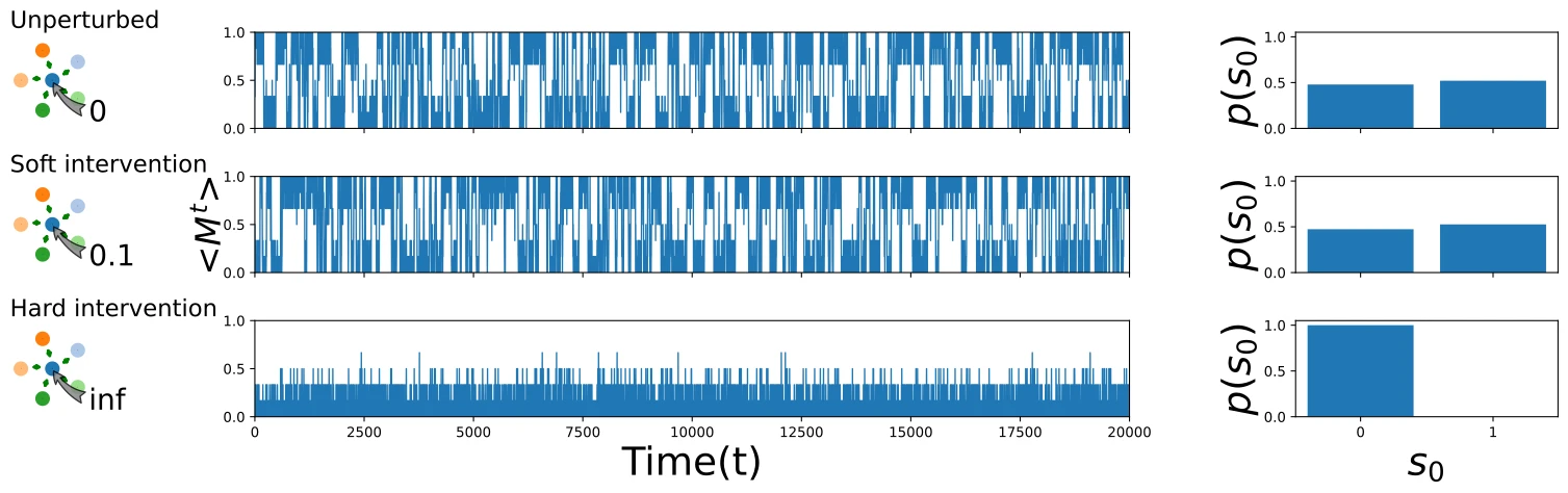
In experiments concerned with measuring causal flows in networks, often “hard” causal interventions are used to determine the causal impact of nodes [79], [80], [81], [82]. Hard causal interventions are those that (effectively) remove all inputs from a node. In contrast, soft interventions, keep the existing causal inputs intact but add an additional causal effect to the dynamics of a variable. In general, the larger the added causal effect of the soft intervention, the more this intervention will “overpower” the existing causal effects and hence the more the soft intervention converges to a hard intervention. In non-linear dynamical systems the intervention size is crucial, since even small interventions can have large effects, especially in the presence of bifurcations. In order to characterize the system without intervention as much as possible, one should thus aim to intervene with a minimal (but still measurable) effect. To illustrate this further, consider the system depicted in Figure 2.2, where each node is update with eq. (2.4). The figure shows the effect of intervention size on the observed system dynamics. Namely, when a hard intervention is used (bottom) the system magnetizes. In contrast, in the non-intervened system, the system magnetizes periodically, i.e. there system dynamics evolve with time periods of magnetization and metastable switches to the other side of the magnetization. Contrasting the non-intervened system (top plot) with the bottom plot (hard) intervention, shows how the metastable behavior disappears. Soft interventions (middle plot) maintain the meta-stable behavior of the system.

There will always be a minimal intervention size for which there is a measurable (i.e. non-zero) causal effect (eq. (2.7)), given finite amount of data. The causal impact will be maximal for hard interventions. As the intervention size is decreased so will causal impact. we hypothesize that there exists a lower bound for the soft interventions for which there will be a measurable causal impact. This minimal intervention size is dependent on the systems structure as well as the dynamics of the system and is difficult to determine a priori. Yet it is important to approach this minimum because if the intervention size is too large, then the intervened system dynamics will diverge from the non-intervened system dynamics, losing its representative capacity. Therefore, we estimate this minimum numerically, described further in Section 2.2.2.

Interventions in kinetic Ising model

In order to measure the causal intervention, transition probability Equation 2.6 needs to be adjusted. For the kinetic Ising model, the transition probability can be modified by adding energy to the node which results in the adjusted Hamiltonian (Equation C.2)

$$\begin{equation} \mathcal{H}_{\textrm{nudge } s_k}(S) = -\sum_{i,j} J_{ij} s_{i} s_{j} - \sum_{i} h_{i} s_{i} - \eta s_i \delta_{ik}. \end{equation}$$(2.8)

That is, an energy term is added to the intervened node $s_k$ by letting it interact with an external ‘spin state’ $\eta$. Both soft and hard interventions were used (see Section 2.1.2). For hard interventions ($\eta \rightarrow \infty$) the nodal dynamics of the nudge node $s_k$ are no longer influenced by nearest neighbor interaction. That is, the node state for the intervened node $s_j$ will not change as a function of time. For soft interventions a grid-search was used with $\vec{\eta} := \{\eta: \eta = 0.55 + i, i\in \{1, \dots, 10 \} \}$ to determine a minimal yet measurable intervention strength. Once determined the same $\eta$ was applied to each node in turn and this process is repeated for all networks in the experiments.

Dynamic Importance Inferred Through Information Flows

Each node in a dynamical system can be considered as an information storage unit [74], [83]. For example in social networks gossip can be considered as information one person possesses. Similarly, disease can be present in one city while being absent in another. Over time through interaction, this information stored in a node will percolate throughout the system while at the same time decaying due to noise. The longer the information of a node stays in the system, the longer it could affect the system dynamics. Therefore, dynamic impact of a node is upper-bounded by the amount of information a node shares with the entire system [74], [75], [84].

How does one measure information stored in a node? A node $s_i$ dictated by stochastic and ergodic dynamics can be considered a random variable. In Shannon information theory information is quantified in bits, i.e. yes/no questions concerning the outcome of a random variable. The average information that a random variable can encode is called entropy and is defined as:

$$\begin{equation} \begin{split} H(s_{i}) = - \sum_{s_{i} = x} p(x) \log p(x). \end{split} \end{equation}$$

Note all $\log$ are base 2 in this chapter unless specified otherwise.

Entropy can also be interpreted as the amount of uncertainty of a random variable. In the extremes the random variable either conveys no uncertainty (i.e. a node always assumes the same state), or is randomly chosen between all possible states (uniform distribution). For example consider a coin flip. One may ask how much information does a single coin flip encode? If the coin is fair, i.e. there is equal probability of the outcome being heads or tails, the amount of questions needed to determine the outcome is exactly 1. In other words, a fair coin encodes 1 bit of information. However, when the coin is unfair the information encoded is less than one. In the extreme case where the coin always turns up heads, the entropy is exactly 0.

The information shared between a node state $s_{i}$ and a system state $S$ can be quantified by mutual information [61], [74], [75], [84], [85]. Mutual information can be informally thought of as a non-linear correlation function which inherits its properties from the Kullback-Leibler divergence. Formally, mutual information quantifies the reduction in uncertainty of random variable $X$ by knowing the outcome of random variable $Y$ [61]:

$$\begin{equation} I( X : Y ) = \sum_{x \in X, y \in Y} p(x, y) \log \frac{p(x, y)}{p(x) p(y)} = H(X) - H(X \vert Y), \end{equation}$$(C.4) where $p(x)$ and $p(y)$ are the marginals of $p(x,y)$ over $X$ and $Y$ respectively, and $H(X \vert Y)$ is the conditional entropy of $X$. The conditional entropy $H(X \vert Y)$ is similar to the entropy; it quantifies the reduction in uncertainty of the outcome $X$ by knowing the outcome of $Y$. Please note that the yes/no question interpretation even applies to continuous variables; although it may take an infinite amount of questions to determine the outcome of a continuous random variable.

Mutual information and causality

Under some contexts, mutual information can be interpreted as being causal. For example for a Markovian, isolated system consisting of two nodes $S = \{s_i, s_j\}$ where $s_j$ causally depends on the previous state of $s_i$, encoded by a conditional probability distribution. It can be readily shown that the causal impact (eq. (2.7)) of $s_i$ on $s_j$ then reduces to mutual information ([61], Section B.II). In this study, the entire system is considered as a downstream node. Importantly, the system is assumed to be measured in its entirety: no confounding variables are allowed. Within this context, the node with the highest integrated mutual information contains more causal information than correlation information than any other node in the system. Since there cannot exist any other node with more mutual information over time by construction of the system, this node must be the driver node. For any other node the measured mutual information can be (significantly) conflated (Figure 2.3). Note that for directed graphs, these methods will not work as by construction the highest mutual information may be lead to wrongful identification of the driver node (see Section B.II).

Additionally, for directed graphs the arrow of time causes a different interpretation on what correlation with the driver node means in cases without unobserved variables (see Section B.II). For $t_0 + t$ where $t > 0$, integrated mutual information may correspond to correlation information of a driver node sender, whereas for $t < 0$, the mutual information relates to the correlation with a driver node sending information. The systems in this study, however, are systems without confounding possessing and undirected network structure. Consequently, information flows symmetrically across the interaction of two nodes and the driver node corresponds to the node with the highest integrated information.

Integrated mutual information

In a network of nodes each causal relation (edge) is obviously not isolated, so confounding variables exist. Therefore, the mutual information between a node state and a future state $I(S^{t_0 - t}; s_i^{t_0})$ cannot be interpreted purely causal in general. Namely, this mutual information could in principle be created purely by another variable $s_j^{t_0 - \omega}$ influencing both $s_i^{t_0}$ and $S^{t_0 - t}$, even if there exists no causal influence from $s^{t_0}$ to any other variable.

Assuming the network itself is isolated, the only node for which the mutual information with a future system state could not have been fully created by a confounding variable is the driver node. That is, the driver node has the largest mutual information with the future system state. If this were fully induced by a confounding variable, then a different node would have to have even larger mutual information with the same future system state. In addition, this must hold for all future system states. By definition of the driver node, this cannot be true under the condition that the system isolated.

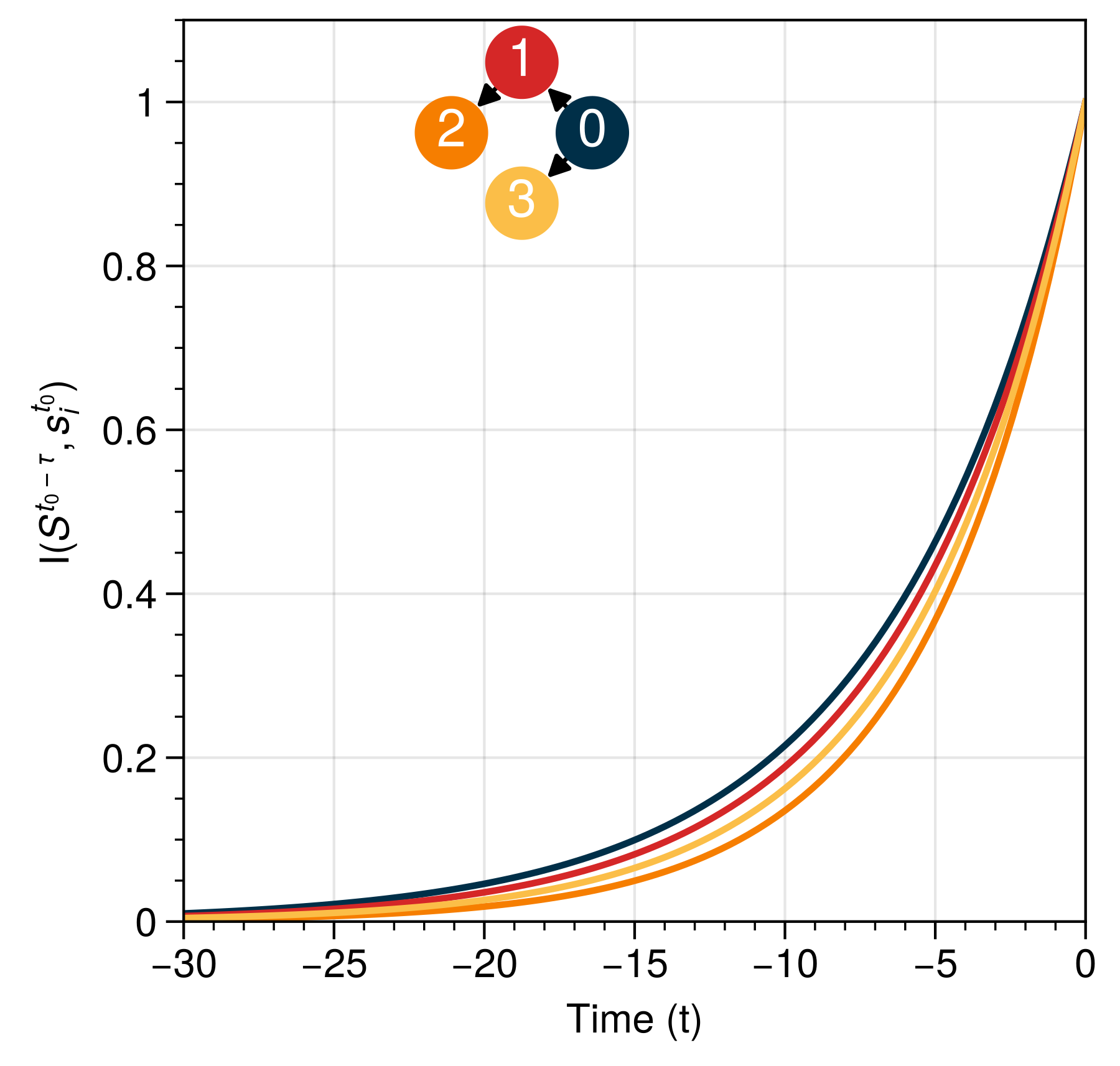
This point is illustrated in Figure 2.3. Note that for all other nodes, however, it is possible for its mutual information value to be inflated due to non-causal correlations. This may result to a non-zero mutual information $I(s_{i}^{t_{0} - t} : s_j^{t})$ among the two variables even if they do not depend on each other in causal manner ( Figure 2.1,Figure 2.2,Figure 2.3). Consequently, we define the integrated mutual information (IMI) for node $s_i$ as

$$\begin{equation} \begin{split} \mu(s_{i}) = \sum^{\infty}_{t=t_{0}} I(s_{i}^{t_{0} - t}; S^{ t_{0} }) \Delta t, \end{split} \end{equation}$$(2.11)

where $S^{t_0}$ is the system state at some time $t_0$ and $s_{i}^{t_{0} - t}$ is the state of a node $t$ away from that system state. At time $t = 0$ the value equals $I(s_i^{t_0}; S^{t_0}) = H(s_i^t)$ for any node.

Here, undirected networks are considered. Due to detailed balance for undirected networks there exists a time symmetry in terms of variable dynamics. This means that for the systems considered in this study $I(s_i^{t_0 - t}; S^{t_0}) = I(s_i^{t_0 + t} ; S^{t_0})$ (see Section B.II). It is computationally easier to compute $I(s_i^{t_0 + t} ; S^{t_0})$ rather than the reverse (see Section 2.2.2). For directed graphs, however, the meaning and interpretation of integrated mutual information changes depending on the direction in time it is computed (see Section B.II). This effect is outside the scope of the present study and will be the subject of future studies. For undirected graphs, the causal impact are time invariant and is equal forward and backward in time.

For all ergodic Markovian systems the delayed mutual information $I(s_i^{t_0 - t} ; S^{t_0})$ will always decay to zero as $t \rightarrow \infty$ [61], [75]. This decay is monotonic, which follows from the data-processing inequality [61] and states that information can never increase in Markov chains without external information injection ( Section B.I). The question is how fast this decay takes place for each node (Figure 2.3), and consequently how much informational impact the node will have on the system.

Taking the entire system as a downstream ‘node’, $I(S^{t+1} ; s_i^t)$ represents pure causal information flow for the driver node as long as there are no confounding variables. For the rest of the study, we will therefore use the notation $I(s_i^{t_0 + t} ; S^{t_0})$.

Methods and Network Generation

Network Data

Synthetic Networks

In total 16 Erdős-Rényi random networks were generated consisting of 10 nodes each. Each random network is generated by first drawing a random connection probability uniformly from [0,1], and then creating each possible undirected edge with probability $r$. Out of these 16 networks, ~82 percent had a single connected component (Figure 2.4). Each edge had unitary weight.

Network of Psychosymptoms

In addition to the generated random networks, we also test a small weighted network inferred from real data. This network differs from the random networks in that it is weighted and reflecting interactions among variables as a consequence of a real-world process, as well as reflecting inferred interactions from real data. The network data originates from the Changing Lives of Older Couples (CLOC) and compared depressive symptoms assessed via the 11-item Center for Epidemologic Studies Depression Scale (CES-D) among those who lost their partner (N=241) with still-married control group (N=274) [86]. Each of the CES-D items were binarized with the aid of a causal search algorithm using Ising model developed by [87] and represented as a node with weighted connections (Figure 2.9 D). For more info on the procedure see [86], [87], [88]. The 11 CES-D items are (abbreviated names used in the remainder of this text in brackets): ‘I felt depressed’ (depr), ‘I felt that everything I did was an effort’ (effort), ‘My sleep was restless’ (sleep), ‘I was happy’ (happy), ‘I felt lonely’ (lonely), ‘People were unfriendly’ (unfr), ‘I enjoyed life’ (enjoy), ‘My appetite was poor’ (appet), ‘I felt sad’ (sad), ‘I felt that people disliked me’ (dislike), and ‘I could not get going’ (getgo).

Numerical methods

Magnetization matching

A prominent feature of the (kinetic) Ising model is the phase change that occurs as a function of noise (Figure 2.4B)[89]. In this chapter we tested whether the amount of noise would (i) affect which nodes becomes the driver node in the system, and (ii) whether the correct driver node could be predicted using either IMI or network centrality metrics. We tested three levels of noise (Figure 2.4 B); a low noise level (80% of the maximum magnetization), a medium noise level (70%), and a high noise level (60%) were used. This magnetization matching was achieved by estimating the magnetization curve as a function of $\beta^{-1}$ numerically.

Estimating $p(S^{t_0})$ and $p(S^{t_0 + t} | S^{t_0})$

For each noise level, $N=\num{1000}$ independent Markov chains are run for simulation with 1000 steps ( Figure 2.4 A). Each chain was initialized with random state distribution over nodes. We are interested in out-of-equilibrium dynamics. For the Ising model the node dynamics are symmetric in equilibrium, i.e. each node has maximum entropy. For any given trajectory, the time-scale for the system to move from a fully magnetized state, to the opposite magnetized state, will take longer than the dynamics that are exerted on local time scales. For short time-scales node with higher degree be more affected by large scale changes in their environment than lower degree nodes. For larger time-scales high-degree nodes will be frozen, and do not reflect short-time scale dynamics. In light of this, the simulations are conducted by sampling one side of the magnetization. This has the added benefit that it reduces the sign of the intervention, i.e. interventions are made to introduce higher entropy in each node which depends on the average magnetization in the system.

Each simulation step executes the following:

1. Pick a node at random from the system with equal probability;

2. Compute energy using eq. (C.2);

3. Flip the node state with probability eq. (2.4).

From this set, the equilibrium distribution over states $p(S^{t_0})$ was constructed in the form of sample of $N$ system states.

For this sample of system states, Monte-Carlo methods are similarly used to construct the conditional $p(s_i^{t_0 + t} \vert S^{t_0})$. For each of the sample states $S_i \in S^{t_0}$, the procedure above was repeated 100000 times for 100 time steps in the psychosymptoms and 30 time steps for the random generated networks. All numerical experiments were repeated $n_{\textrm{trials}} = 20$ times to provide confidence intervals for the results in all nudge conditions and temperature settings (noise conditions).

Time symmetry and mutual information

Thusfar, the definition of causal impact and IMI is ambiguous to the whether $t$ is positive or negative. Namely, if the node state $s_i^{t \pm 1}$ is captured in forward in time or backward in time with respect to some state $S^{t}$. For undirected networks with Ising spin dynamics there exists time symmetry with respect to how causal influence flows through the network due to detailed balance (see Section B.II). However, for directed networks this is not the case. The results obtained here are obtained using forward simulation in time only. The detailed balance condition ensures that the results would be symmetric when simulating the system backwards in time.

Area under the curve estimation

The mutual information over time and KL-divergence over time were scaled for visual purposes in the range $[0,1]$ per trial set. A double exponential, $y = a \exp(-b (t - c)) + d \exp(- e(t - f) )$, was fitted to estimate these curves and subsequently IMI (eq. (2.11) and (2.7)) using least squares regression ( Figure 2.7,Figure 2.9 C). The kernel showed to be a good fit as indicated by the low fit error ( Figure B.III.1a, Figure B.III.1b).

Sampling bias correction

Empirical estimates for mutual information are inherently contaminated due to sampling bias. In order to correct for this, Panzeri-Treves correction was applied [90]. This method offer a good performance in terms of signal-to-noise and computational complexity.

Driver node prediction and precision quantification

It is possible for two or more nodes to have exactly equal network structure features as well as node dynamics. For example consider a ring structure where each node has the exact same connectivity and all nodes have the same dynamics. In this case each node must have the same causal effect, and it would be impossible to disentangle these nodes causally from one another. Similarly graphs that are similar, e.g. show high degree of structural similarity but are not isomorphic, this causal separation may proof difficult for finite samples in stochastic settings as was discussed in Section 2.2.2. Consequently, we applied a parametric bootstrap procedure to estimate driver node sets (algorithm (B.VII.1)).

Driver set estimation

The area under curve values, e.g. integrated mutual information and causal impact, were resampled to generate bootstrap distributions (Section B.VII). This creates a confidence interval for the integrated mutual information and causal impact. From these bootstrap distributions a driver node set is estimated (see algorithm (B.VII.1) in Section B.VII). The bootstrap procedure constructs driver node set $\Lambda$ iteratively by comparing the overlap $\phi$ with of the bootstrap for each variable with the distribution of the estimated driver node. For all experiments $\phi = 0.5$. The driver node distribution was taken as the bootstrap distribution with the highest mean. Variables will be included to the driver node set $\Lambda$ if the overlap between its bootstrap distribution $i$ and driver node bootstrap distribution $j$ was $\phi_{ij} > 0.5$. In total $N = 1e4$ bootstrap trial were constructed of size $M = n_{\textrm{trials}} = 20$; for each of the trials the average was computed. For each variables a Gaussian distribution was estimated over the $N$ bootstrap. This distribution was used for computing the overlap with the driver node distribution.

The bootstrap procedure cannot be applied to the network centrality metrics as there exists only one centrality rank assignment per network structure. Therefore, the driver nodes as inferred by maximum centrality metrics is the set of nodes ($\Lambda$) whose centrality metric ($f$) equals this maximum value, i.e.

$$\begin{equation} \begin{split} \Lambda_{cent} = \textrm{argmax} f_{cent}(x) := \{ x \in S : f_{cent}(s) \leq f(x) \forall s \in S \} \end{split} \end{equation}$$(2.12)

where $f$ is the centrality function which assigns a real value to each node in the system. For degree centrality,

$$\begin{equation} \begin{split} f_{deg}(a_i) = \sum_j a_{ij} \end{split} \end{equation}$$

where $a_{ij}$ is the weighted connectivity between node $i$ and $j$ in the adjacency matrix $A$ of the network. If $a_{ij}>0$ node $i$ and $j$ are connected. In this study degree, betweenness, closeness or eigenvector centrality were used. (see Section B.VI for the formal definitions for the centrality measures).

Ground truth comparison

The ground truth values are the driver node estimations for the causal impact bootstrap distribution. Each estimator also generated a driver node set estimation. That is for integrated mutual information, degree centrality, closeseness centrality, betweeness centrality, eigenvector centrality, the bootstrap distribution generates an estimated driver set. To evaluate the performance of these estimators, an overlap score was computed with the ground-truth (causal impact estimation) using the Jaccard similarity metric:

$$\begin{equation} J = \frac{A \cap B}{A \cup B}. \end{equation}$$(2.14)

A Jaccard score of 1 means perfect overlap, i.e. the driver node set identified by causal impact and predictor set by IMI or one of the centrality metrics are identical. Conversely, a Jaccard score of 0 means completely disjoint driver-sets.

For every network, intervention size and temperature the similarity metric we computed the Jaccard score per predictor. Additionally, the relative performance ratio of the IMI predictor was evaluated by

$$\begin{equation} \begin{split} R_{cent} = J_{IMI} - J_{cent} \end{split} \end{equation}$$(2.15)

where $J_{cent}$ is the Jaccard score of the structural metrics (betweenness, closeseness, betweeness, eigenvector centrality). This performance indicator falls within [-1, 1] range: A value of -1 would indicate that the centrality metric correctly identified the driver node set; a score of 0 would indicate equal performance for the driver node identification between a centrality metric and IMI; a score of 1 would indicate a correct identification of the driver node for IMI, but a false identification of the centrality metric. The ratios were bootstrapped ($N = \num{100 000}$) and tested for significance at $\alpha = 0.01$. The driver node inferred performance is bound between $(0, \infty)$.

The Effect Of Intervention Size on Observed Dynamics

Understanding the accuracy of these methods is crucial for identifying influential nodes that drive system dynamics, which has broad applications. We first focus on evaluating the performance of IMI as a predictor for the driver node in dynamic networks with a synthetically generated network structure. Following, we will apply the methods to a real-world generated network.

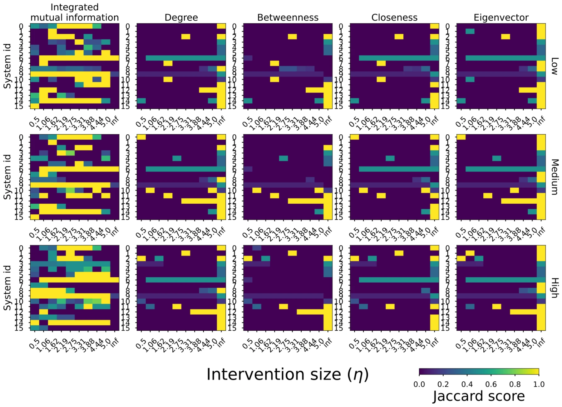
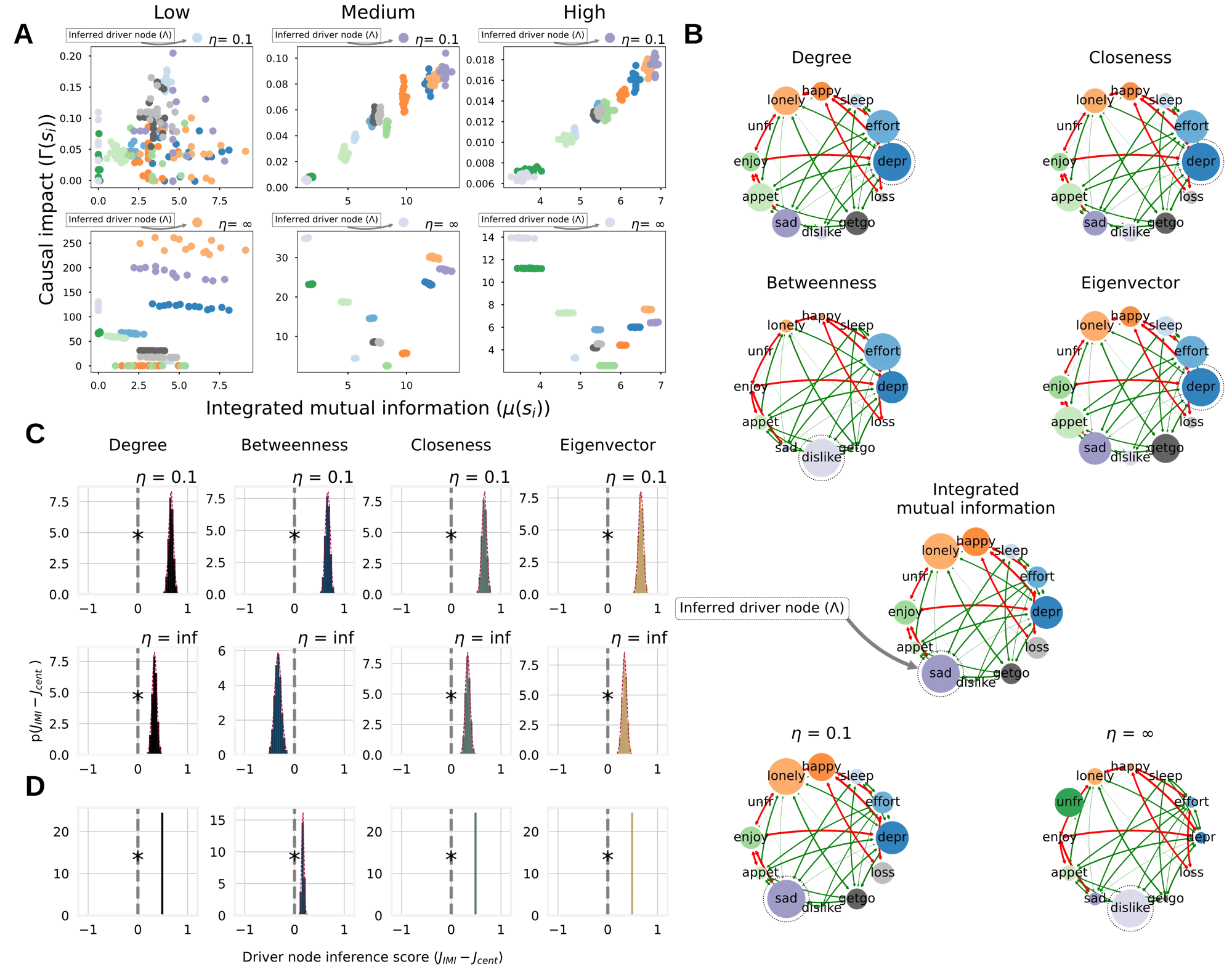
Driver node inference accuracy is depicted in Figure 2.5 for both IMI and the network centrality measures. Three crucial observations can be made from the Jaccard scores.

First, for nearly all systems there exists an intervention size for which IMI obtains a Jaccard score of 1 (perfect true driver node inference), whereas this is not always the case for the centrality metrics, see e.g. system 3, 7, 15.

Secondly, IMI is predictive nearly only for soft intervention sizes, i.e. intervention sizes smaller or of similar order of magnitude as the existing forces acting on nodes(i.e. their degree in the $J$ interaction matrix).

Lastly, centrality metrics are mainly predictive for hard interventions. The statistical results reflect these observations (Figure 2.8 A and B).

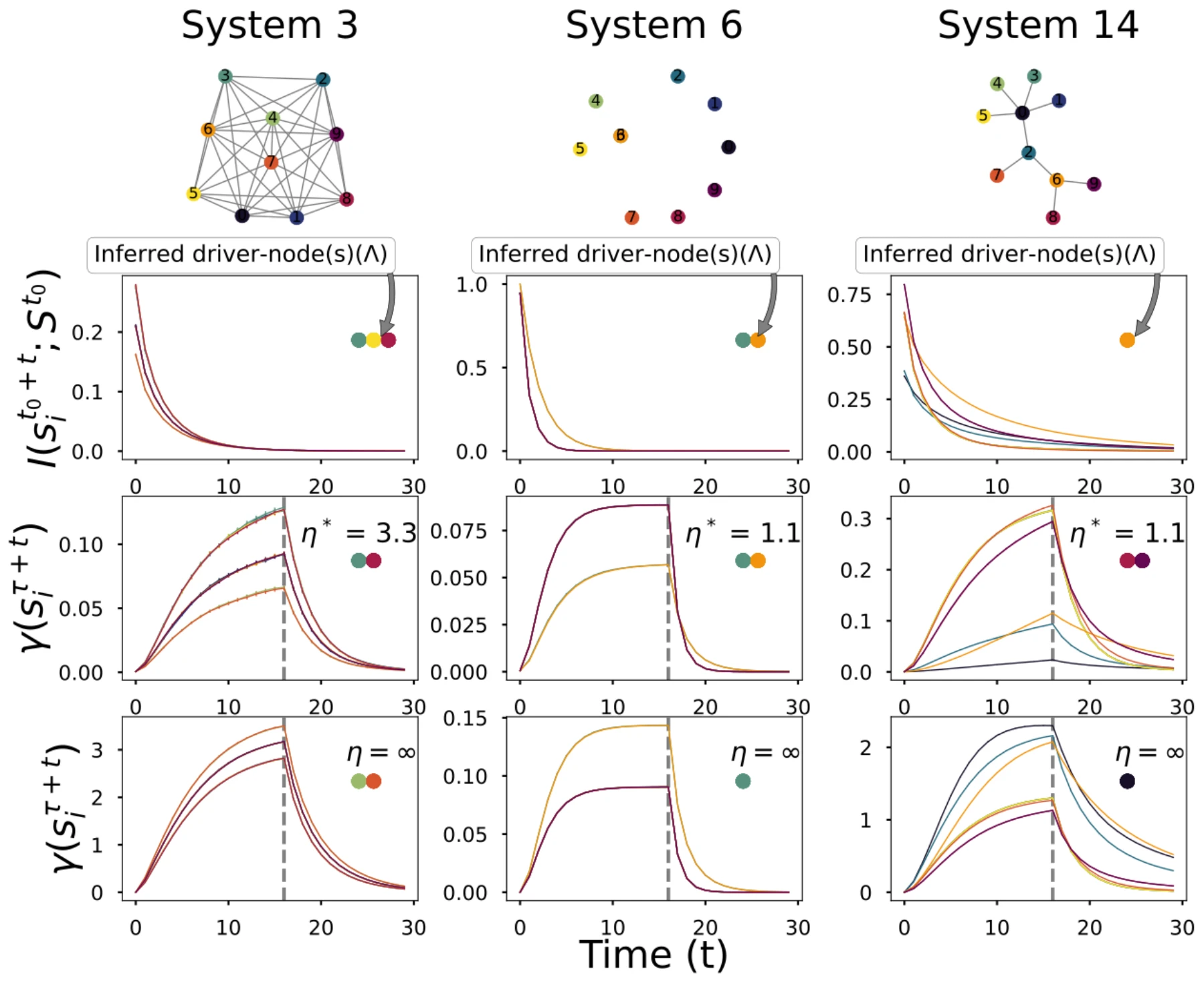
In Figure 2.6, average decay curves are shown for IMI (top) and different intervention sizes (middle) as well as hard interventions (bottom) for systems 2, 5, and 12. The network structure of these systems is depicted in Figure 2.6 (top). Notably, comparing the hard interventions (bottom) with a more moderate intervention strength (middle) in system 2 reveals that the driver node can significantly differ depending on the intervention size applied to the system. Furthermore, the order of causal importance is noticeably different for the minimal intervention $(\eta^*)$ versus the strong intervention $(\eta=\infty)$ (middle and bottom plots in Figure 2.6).

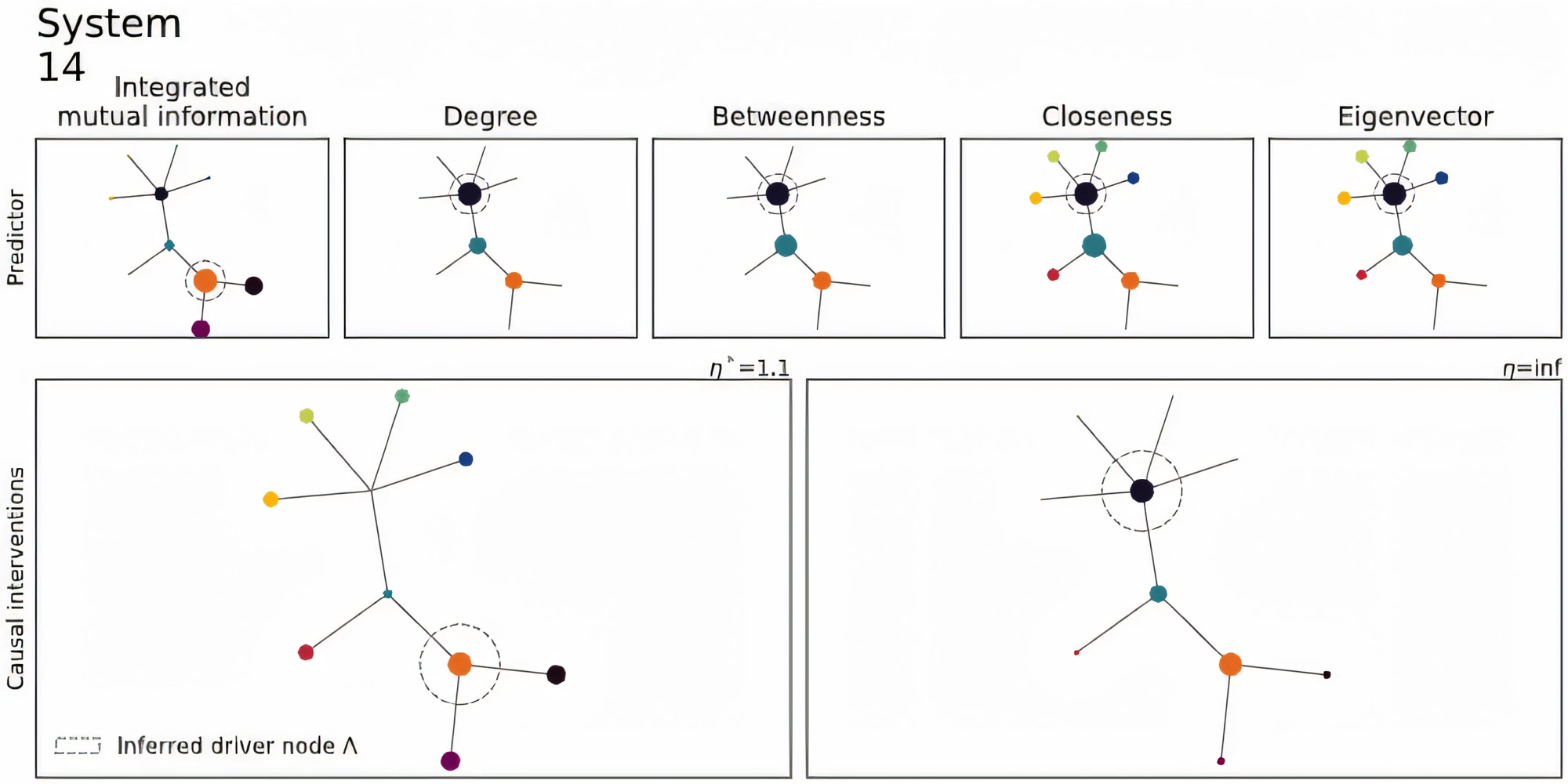
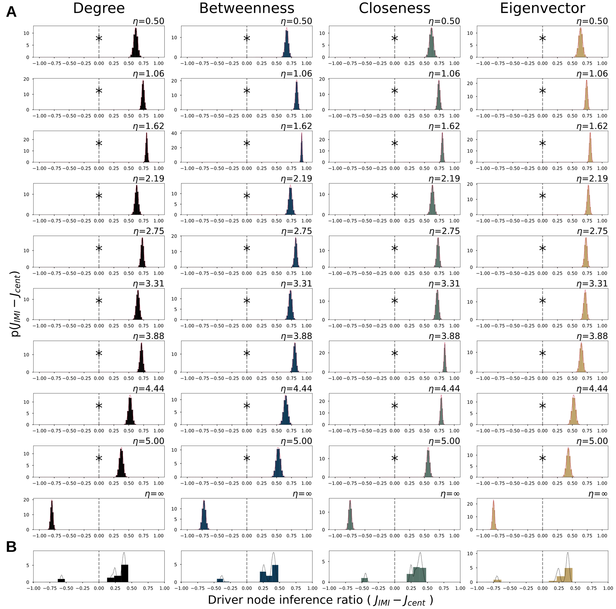
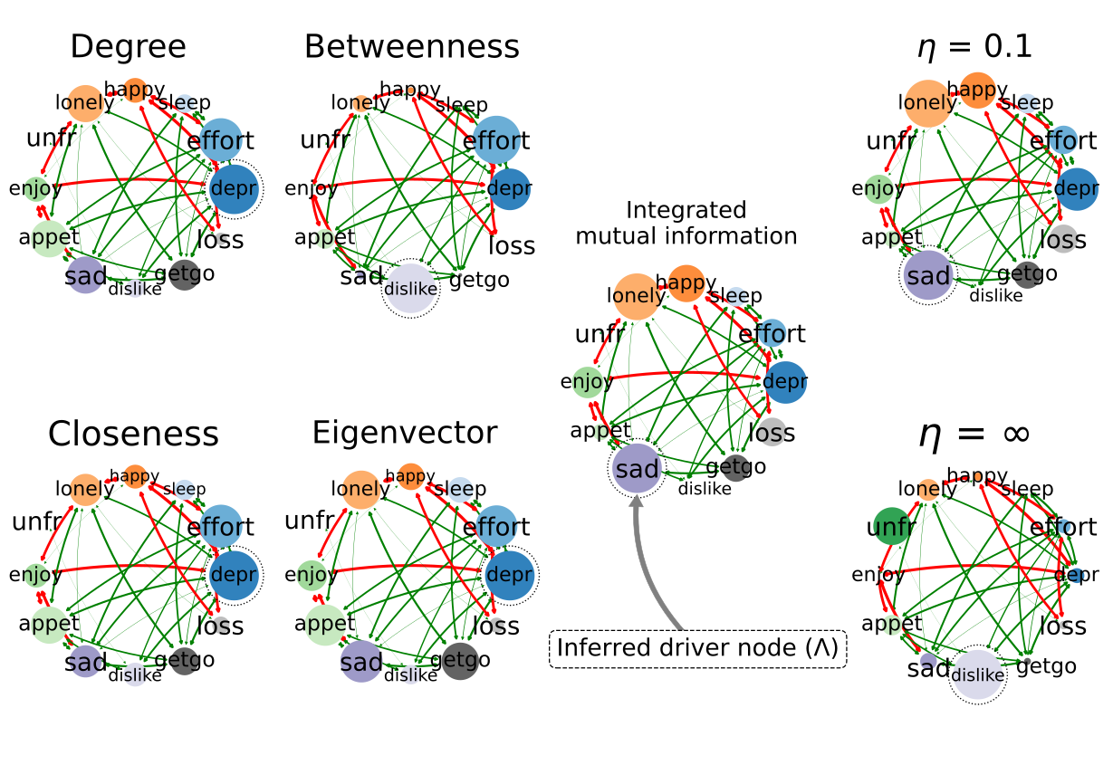
The real-world system, encompassing a network of psychological symptoms, exhibits results analogous to those observed in random networks as depicted in Figure 2.9. Specifically, at medium to high noise levels, the IMI consistently yielded significantly higher Jaccard scores compared to centrality metrics under low causal interventions (Figure 2.9 C/D; $p << 0.01$), although this was not the case for hard interventions. Conversely, hard interventions led to entirely distinct causal structures that did not align with the dynamics of the non-intervened system (Figure 2.9 A/B). For instance, under hard interventions with medium and high noise, “dislike” was identified as the primary driver node (Figure 2.9 A), whereas in cases of low causal intervention, ’sad’ took on that role (Figure 2.9 A). This suggests that interventions can significantly influence the observed causal structure and may reveal systemic behaviors not evident in the non-intervened system. Notably, soft interventions with $\eta = 0.1$ proved insufficient to discern driver nodes under low noise conditions (Figure 2.9 A). Furthermore, hard interventions in low noise scenarios identified a different driver node compared to softinterventions. The grid search for a optimal $\eta^*$ was inadequate for the psychosomatic network and requires further investigation in future studies.

In addition, the change in driver node observed in Figure 2.9 A highlights one major flaw in centrality metrics: they cannot account for a change in driver nodes due to a change in dynamics. The implicit assumption on dynamics that each centrality metric holds, provides only one estimate per network structure. In contrast, IMI does not depend on what mechanisms generate system dynamics. Instead, it uses the distribution dictated by these system dynamics which match the true driver nodes.

Fried and colleagues postulated that ‘lonely’ was the gateway from which information spreads through the network, i.e. bereavement was embodied mainly by ‘loneliness’ which then percolated its effect to the other symptoms [86]. Since the data was cross-sectional, the comparison with the results from this study relies on the assumption that binary dynamics are representative of the absence and presence of psychological symptoms. If correct, the results from this study give a causal perspective on the associative results from [86]. The results from this study postulate that ‘depr’, ‘lonely’ and ‘sad’ have similar causal effect for moderate to high thermal noise.

It is important to emphasize that a quantification is given in terms of absolute effect size and not directed effects. This means that nudging for instance ‘sleep’ has some effect $X$ on the psycho-symptom network, in what direction that effect is, or whether it has a positive or negative effect on the bereavement score / cognitive load of the patient is not clear, and should be the subject of future studies (see Section B.IV).

When Structure Meets Behavior: The Dance of Complex Systems

Structural metrics can be considered as implicitly assuming a particular dynamics [91], [92]. For example, the eigenvector centrality has a clear analytical connection with linear dynamics, such as a simple diffusion process. Betweenness centrality on the other hand can be considered to assume that causation between nodes is transmitted mainly along the shortest paths between pairs of nodes (see Section B.VI), such as in message or package routing. Finally, many more network centrality metrics have been developed based on specific dynamics, such as current and flow centrality measures. Thus, such network structural metrics could indeed be used, but a careful analysis of the dynamic equations is required to assess which centrality measure (if any) turns out appropriate.

The results from this study show that high degree nodes with Ising spin dynamics tend to actually not be a driver node for small interventions. In this model it can be understood since high degree nodes exhibit “frozen” behavior; their large(r) number of neighbors effectively sum up to a constant and strong force towards the majority state. Consequently, a constant (soft) intervention will be relatively ineffective with hubs. For non-intervened Ising dynamics, it makes intuitive sense that the dynamics are driven by the nodes which are neither “frozen” (hubs) nor are poorly connected (low-degree nodes), which is reflected by the soft intervention setting. This insight is specific to the Ising system but illustrates that the information flow and causal flow of a system is not merely determined by the connectedness of a node in the network. Rather, the connectedness of the entire system in addition to inter-node dynamics combined are crucially important for causal flows and driver node identification.

The results further imply that for unperturbed dynamics structural metrics may not be predictive for determining the causal importance of nodes. Soft interventions revealed different causal structure than hard interventions ( Figure 2.5 Figure 2.9). For hard interventions, structural metrics do become predictive for causal importance for the networks studied here. However, the dynamics of these systems are shown to deviate from the non-intervened dynamics, causing system dynamics that are not representative of the non-intervened system. This can be seen in the causal influence in Figure 2.5 and Figure 2.9 where the causal influence for hard interventions is opposite to soft causal interventions. Consequently, if the aim is to provide understanding to the information flows for non-intervened dynamics, then hard interventions are not preferred.

In addition, the results imply that in order to achieve maximum impact for a fixed ‘intervention’ budget (injected energy), choosing the high degree nodes is not necessarily optimal. The adjusted Hamiltonian (eq. (2.8)) introduces a bias on low degree nodes. Here, a causal intervention was performed by adding fixed energy to the Hamiltonian. For fixed intervention size $\eta = c$, the causal impact on the nodal distribution will be relatively higher for nodes with low degree than nodes with higher degree. Higher degree nodes may have higher causal effect in principle if the same probability mass is changed. However, moving the same probability mass scales non-linearly in kinetic Ising (eq. (C.2)). For a limited ‘intervention budget’ it is preferred to locate those elements of the system that reaches maximal causal effect.

For, some systems, however, the inferred driver node never matched the true driver node(s) (e.g. system 8 in Figure 2.5). This could be due to two main reasons. First a grid-search was applied for the intervention size. It was argued that there would be a minimal intervention $\eta^*$ which would lead to a measurable effect. It is possible that the parameter space used here missed the intervention size that provided enough resolution to accurately determined the driver node(s). Second, the numerical procedure for driver node inference could be optimized. The overlap of distribution was set to $\phi = 0.5$, to infer the driver node set $\Lambda$, to prevent false positives for driver node identification due to noise in observed system states. However, the choice of parameter was not optimized and could lead to ambiguous driver node inference. System 8 in particular was most nodes in the network had a similar connectivity pattern, and as such causal isomorphy occurs, i.e. the causal importance of a node is indistinguishable from any other node in the system. The bootstrap estimates led to high level but not perfect of overlap (see Section B.VII). Consequently, if $\phi$ was set differently, the inferred driver nodes could be improved. In future studies, we aim to further look into what how this numerical procedure could be improved for inferring driver nodes in dynamical networks particularly for causal isomorphic nodes.

Limitations

The systems considered are discrete and ergodic. IMI assumes that the data-processing inequality holds for the system (Section 2.1.3). The data-processing inequality in ergodic systems ensures that $I(s_i^{t_0 + t} ; S^{t_0})$ monotonically approaches zeros as $t \rightarrow \infty$ (see Section B.I). As a consequence IMI will always be finite for ergodic systems. For non-ergodic systems, the data-processing inequality can only guarantee that $I(s_{i}^{t_{0} + t} ; S^{t_{0}})$ never increases as a function of $t$. Namely, the data-processing inequality ensures that no local manipulation of information may increase the information content of a signal. This implies that as $t \rightarrow \infty$, IMI may not converge for nodes with non-zero baselines. For these non-ergodic systems, however, it may be possible determine the driver nodes by considering finite time-scales, or subtracting the asymptotic $\gamma$ value and reporting it separately.

Furthermore, this study only considered information flows undirected systems. For directed systems, the largest integrated mutual information may in fact not be the driver node due to correlation. In Section B.II an integrator is node is considered, where the integrator stores the system information but lacks any causal outgoing connections. The information storage capacity in this node will be higher than any other node due to its increased alphabet. If this integrator node encodes a copy operator, its information decay will result in the highest integrated mutual information while lacking any causal potential. In the systems considered here, this situation cannot occur. That is, for undirected systems information flow has equal potential along an edge. Any causal effect a node has in undirected dynamical systems, will percolate to all neighbors of a node. For directed graphs the information flow is not time symmetric as detailed balance cannot be ensured. Consequently, the use of forward mutual information $I(s_i^{t_0 + t} : S^{t_0})$ may lead to false estimates of driver nodes in these cases. For undirected graphs, if there would exist a node with higher integrated mutual information, its causal impact will also be higher and as such it would be the driver node. The asymmetry of information flow, and the compound nature of both correlation and causation restricts the use of integrated information undirected graphs.

In addition, the focus on short-time scales biases information processing to less constrained nodes. By measuring the system out-of-equilibrium, the system dynamics for the kinetic Ising model has the tendency to “freeze” the behavior of nodes as a function of increasing degree. For undirected systems, this assumption seems sensible as the higher causal potential for hubs forms at the same time a higher constraint for switching its state. The flip probability of node $s_i$ in the kinetic Ising model as a function of degree will tend to zero given that the neighborhood is congruent with the node’s current state. Measuring the system in equilibrium, will therefore result in nodes with higher degree to have lower information decay. In contrast, out-of-equilibrium a node state will have lower variability and consequently less causal effect on the instantaneous system states. Therefore, the driver node identification through integrated mutual information are only valid for non-equilibrium kinetic Ising spin dynamics with undirect network structures. Since the Ising spin dynamics falls within a larger universality class, such as (directed) percolation. This implies that the results from this study may apply to different dynamical systems sharing the same core assumptions.

Systems of size at most $(n=12)$ were used. The size of the system was chosen due in order to provide high reliability of the probability distributions. In addition, larger graphs can be decomposed in various different network motifs [76]. It is believed that these motifs form the “computational” buildings blocks for larger complex systems under the assumption of nearest neighbor interactions. That is, understanding the motifs would gain insights in how a macroscopic property emerges from local interactions. The aim of this study was to relate structural connectedness to dynamic importance; the exact nature or occurrence of motifs were not the focal point. In real-world systems, however, it is exactly the composition and interaction of these motifs that are vital to complex systems. Here, the motifs were implicit on the real-world network and the generated structures. I leave it up to future work to map out the driver nodes of common network motifs in different dynamics and relate the structural importance to the dynamical importance.

The Dynamic Importance of Nodes is Poorly Predicted By Static Topological Features

Our results indicate that dynamic importance cannot necessarily be reliably inferred from network structural features alone, demonstrated here using kinetic Ising spin dynamics. The goal of this chapter was to show that structural methods can provide unreliable estimates of the driver node in dynamical systems. The results from this study show that the common assumption of structurally central or well-connected nodes being simultaneously dynamically most important is not necessarily true. This implies that we cannot abstract away the dynamics of a dynamic system before inferring driver nodes. The proposed information theoretic metric, integrated mutual information (IMI), was better able to identify the driver node for non-intervened dynamics in systems. Importantly, IMI does not require knowing the dynamics equations and/or the network structure of the system. It is instead calculated directly from a cross-section of time-series of the system without interventions. The proposed metric could potentially be useful in applications with rich data sets and where performing interventions are infeasible or impractical.

In essence, our findings echo Frank Lloyd Wright’s assertion that “Form follows function – that has been misunderstood. Form and function should be one, joined in a spiritual union." Similarly, in complex networks, structure and dynamics are inextricably linked, forming a unified whole. Just as Wright advocated for a harmonious blend of form and function in architecture, our work underscores the importance of considering both structural and dynamic aspects when analyzing complex systems. By embracing this holistic approach, we can gain deeper insights into the true nature of driver nodes and the underlying mechanisms that govern system behavior.