How to Intervene?

Numerical Methods

Graph Generation and Link density, and Assortativity

For the Monte-Carlo results, graphs were generated by spawning a ring with $Z=150$ in which each role was alternating ensuring that the base graph would have maximum assortativity, with minimum degree. Furthermore, this ensured that each role occurred equally ($Z_r = 50 \forall r \in R = 1, \dots 3$)

The link density was increased by adding new edges between agents of non-matching roles. That is, only edges were added if the two roles did not share the same role. This would ensure that the assortativity for the base graph would not increase with the number of edges added. the link density was increased from the base ring by a fraction $f \in \{0, 0.1\}$ in 5 equally sized steps. This range was determined by first evaluating up to $f=1$, and seeing that above 0.1, the values don’t increase much further.

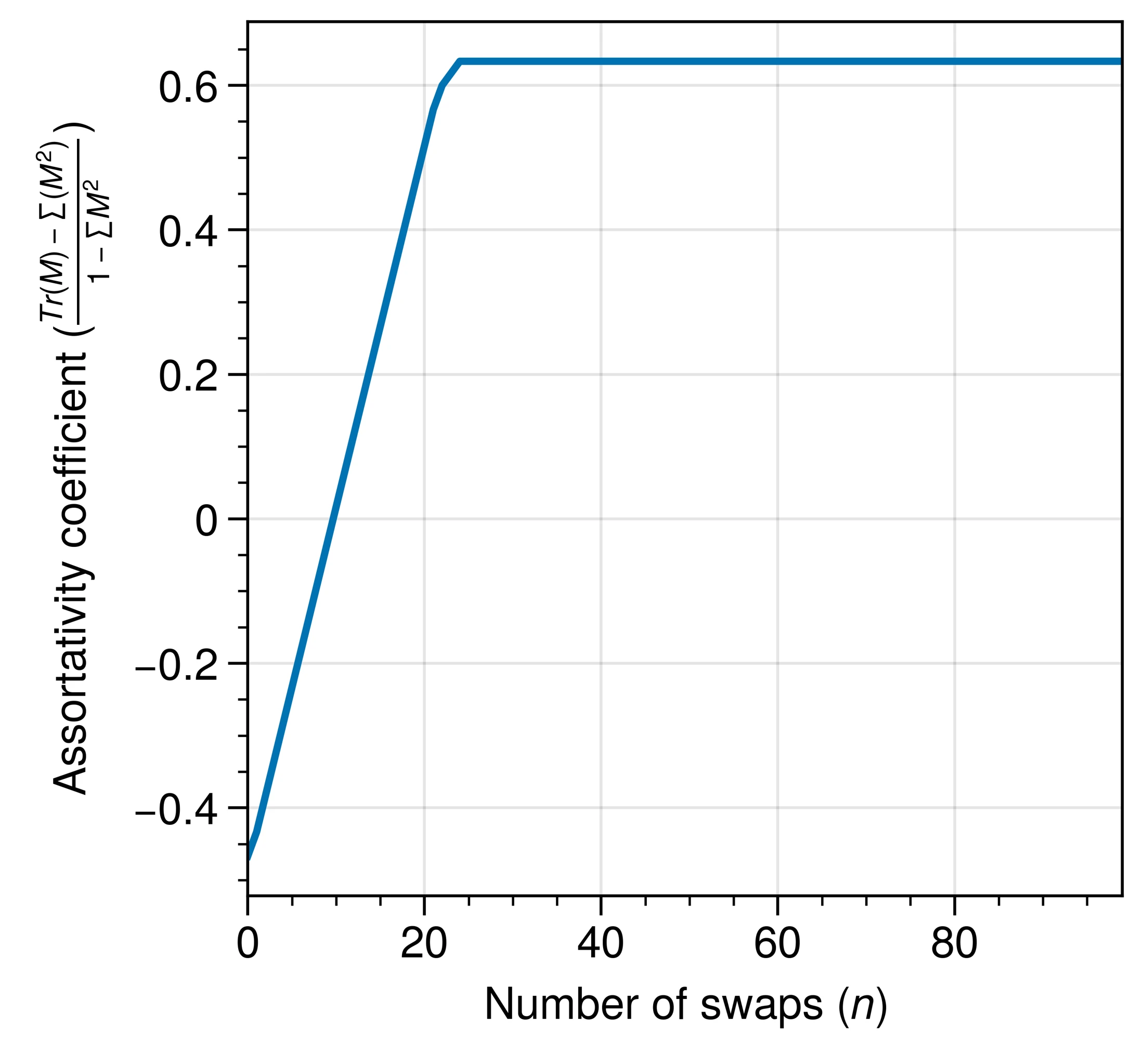
Assortativity was increased by considering $n$ swaps such that the assortativity $q$ would increase to $q'$, this was performed using exhaustive search. Only graph edits were allowed that increased the assortativity. The number of swaps was varied between the range $[0, 100]$ with dynamic step size. The range $[0, 10]$ was sampled densely, after the number of swaps increased by increments of 5 (until 20), and 10 (>20). The assortativity coefficient for graph $G$ for the roles as attributes as:

$$\begin{equation} A_G = \frac{Tr(M) - \sum(M^2)}{1 - \sum M^2} \end{equation}$$(D.1) where $M$ is the joint probability distribution or mixing matrix [244].

Monte-Carlo Simulations

The effect of link density (Section 4.4) were performed using Monte-Carlo methods. The maximum incurred costs (D.I.3) was computed using bisection search. This was achieved by starting the simulation from a state were all agents were criminal or non-criminal and then stepping the system for $T = 1000$ steps. The final state was used to estimate the fixed point by computing the average state of the nodes in the system. Each simulation step, consists of updating all the nodes in the system ($Z = 300$) in random order.

The model was written in Nim (version 2.0). Random numbers were generated using the xoroshiro128+ generator provided by Nim’s standard library. Visualization and data-analysis was performed in python using Matplotlib. Source code is available at https://github.com/cvanelteren/boiler_room.

Numerical Validation of Phase Diagram

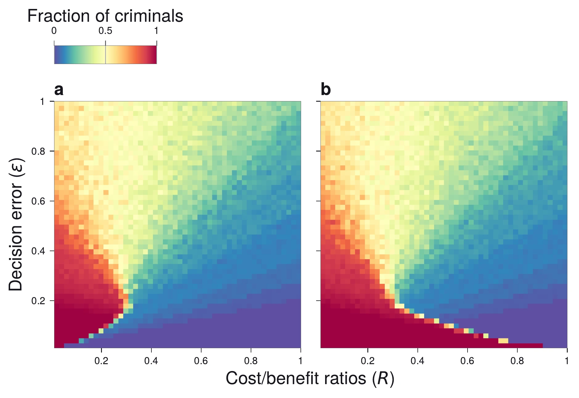
Using the methods described in D.I, we replicated the results analytical results shown in Section 4.2. For the Monte-Carlo simulations we choose the number of local samples to be $n = 100$ for each agent which is shown to converge closely to the analytical solution (Section 4.5). The Monte-Carlo results on complete graphs show close similarity to the analytical result(Section D.I.2)

Criminal Robustness: Incurred Cost

We defined maximum incurred cost as the maximum cost for which a criminal organization can be formed. For a given noise value $\beta$, we hypothesize that the networks can nurture or deprive conditions to form criminal organizations. Let $S^t = \{s_1, s_2, \dots, s_z\}$ indicate the (criminal) state of the agents at time $t$, then we can write the criminal robustness by its maximum incurred cost as

$$\begin{equation} c^*(\epsilon, \langle S^0 \rangle = 1) = \max_c \langle S^t\rangle \neq 1. \end{equation}$$(D.2)

We are interested at which cost $c^*$ the system has only 1 stable attractor. In other words, at which cost, does the system loose its ability to sustain a saturated criminal market.

The maximum incurred cost is evaluated for networked systems numerically through bisection search. Simulation were performed starting with all agents in the criminal state $\langle S^0\rangle = 1$. Since the maximum inccured cost depends on the noise level, care was taken into choosing a proper value such that there exists a stable point for a saturated criminal market. The result from Section 4.2 was used to determine a value for $\beta$. The analytical results form an upper bound for networked systems. That is, the network structure will impose constraints on the ability to reach a saturated market for a given noise level; it cannot improve over the well-mixed conditions As such it was determined that $\epsilon = 10$ was used to compute $c^*$ for the networked systems.

The simulation time was set to $t=300$ using the same update settings as described in D.I.2.

Criminal Opportunity

Criminal opportunity is defined as the instantaneous number of criminal organization out of all possible organizations at the end of a simulation, or

$$\begin{equation} O^t = \sum_{i=0}^Z \frac{M_i^t}{\mathcal{M}_i^t}, \end{equation}$$(D.3)

where $M_i^t$ are the number of criminal organizations for agent $i$ at time $t$ and $\mathcal{M}_i^t$ indicates the total organizations agent $i$ could have formed at time $t$.

Derivation of Section 4.1

Section 4.1 describes the payout of a singular game. We consider the change of the three subpopulations as a stochastic variable. Let $x_r$ describe the fraction of criminal of each role $r \in R$ in the population, then the expected payout $r$ becomes

$$\begin{align*} \pi_r = (1 - x_r) \sum_{k = 0}^n (\prod^R_{j=0, j \neq i} x_{j})^k (1 - \prod^R_{j=0, j \neq i} x_{j})^{n - k} \frac{1}{1 + e^{-\frac{1}{\epsilon}(kb \prod^R_{j=0, j \neq i} x_{j} - cn)}}. \end{align*}$$(D.4)

Following, we can describe the instantaneous change of the system as the balance between the gains and losses of a criminal in a particular role $x_r$. We can write:

$$\begin{align} \frac{d}{dt} x_i &= \mathbb{E}[x_i^+] - \mathbb{E}[x_i^-] \\ &= (1 - x_i) \sum_{k=0}^n \binom{n}{k} \left( \prod_{\substack{j=0 \\ j \neq i}}^R x_j \right)^k \left(1 - \prod_{\substack{j=0 \\ j \neq i}}^R x_j\right)^{n-k} \frac{1}{1 + e^{-\epsilon \left( \frac{k}{n} b - c \right)}} \nonumber \\ &\quad - x_i \sum_{k=0}^n \binom{n}{k} \left( \prod_{\substack{j=0 \\ j \neq i}}^R x_j \right)^k \left(1 - \prod_{\substack{j=0 \\ j \neq i}}^R x_j\right)^{n-k} \frac{1}{1 + e^{-\epsilon \left( \frac{k}{n} b - c \right)}} \nonumber \\ &= \sum_{k=0}^n \binom{n}{k} \left( \prod_{\substack{j=0 \\ j \neq i}}^R x_j \right)^k \left(1 - \prod_{\substack{j=0 \\ j \neq i}}^R x_j\right)^{n-k} \left( \frac{1 - x_i}{1 + e^{-\epsilon \left( \frac{k}{n} b - c \right)}} - \frac{x_i}{1 + e^{-\epsilon \left( \frac{k}{n} b - c \right)}} \right) \nonumber \\ &= \sum_{k=0}^n \binom{n}{k} \left( \prod_{\substack{j=0 \\ j \neq i}}^R x_j \right)^k \left(1 - \prod_{\substack{j=0 \\ j \neq i}}^R x_j \right)^{n-k} \frac{1}{1 + e^{-\epsilon b \left( k - \frac{c}{b} n \right)}} - x_i. \nonumber \end{align}$$(D.5)

In the limit of $n \to \infty$, section Section D.5 can be written as $$\begin{equation} \begin{split} \lim_{n\to\infty} \frac{d}{dt} x_i = \frac{1}{1 + e^{- \frac{1}{\epsilon} b(\prod_{j = 0, j \neq i}^R x_j - \frac{c}{b})}} - x_i, \end{split} \end{equation}$$ see [245] for proof.

The model formulation is akin to a n-order Ising model with base $\{0, 1\}$ under transversal magnetic field where each agent takes local averages [246].

Role Diversification Drives Bifurcation

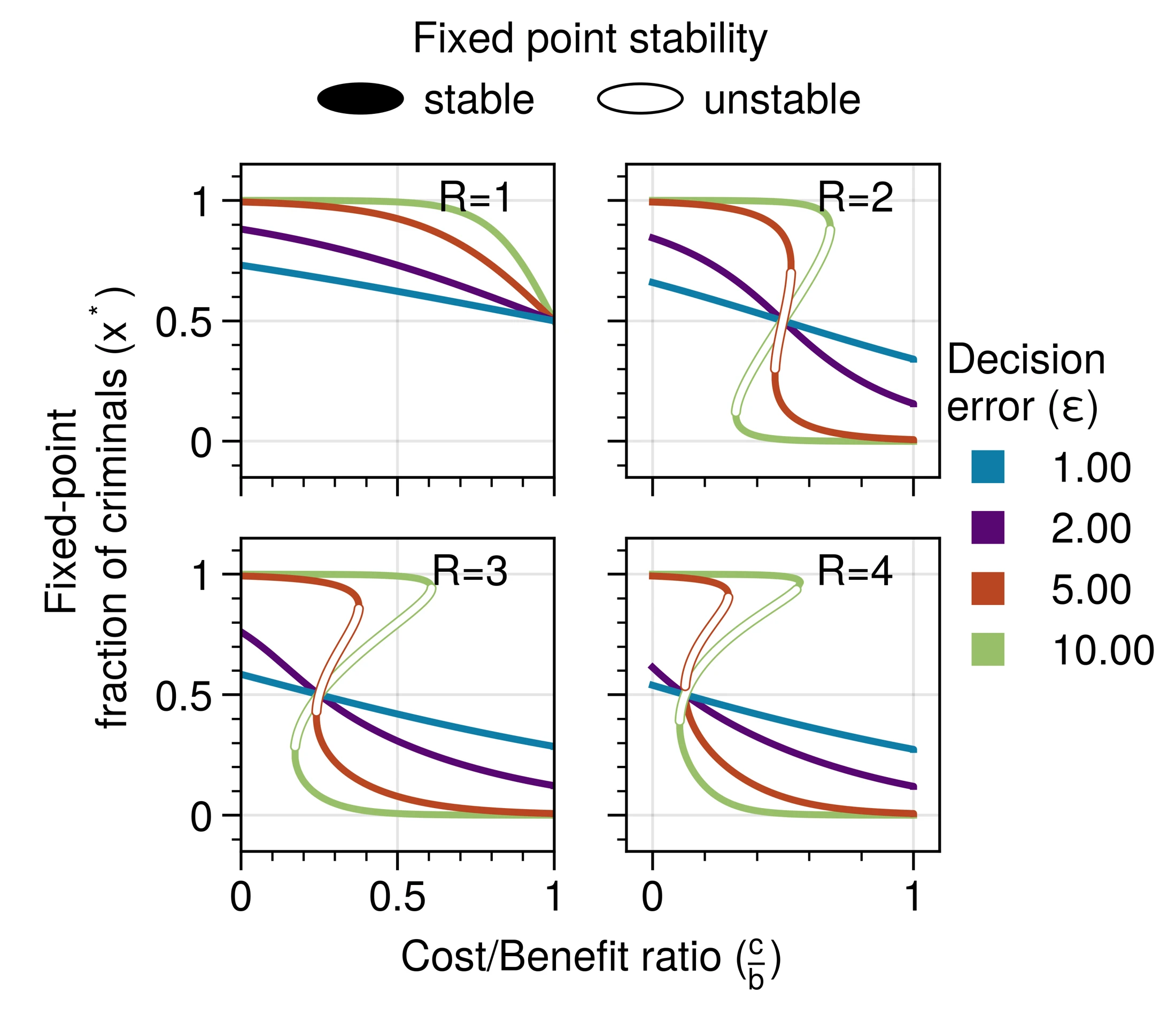
For lone wolf criminals (Section D.III.1, top left), (4.3) implies the existence of a singular stable point as a function of the benefit ratio and given noise value. Noise affects the dynamics of system by sharpening (or soften) the sharpness of the curve. For high noise conditions, criminal strategy becomes random (50/50) whereas for lower noise values, the criminal strategy becomes favorable for high benefit $b$.

For $R \ge 2$, a bifurcation emerges. As the cost decreases past a critical point ($\frac{c}{b} \approx 0.5$), an unstable fixed point occurs flanked by two stable fixed point; one in which a high level of criminal activity is present, and another in which the criminal activity vanishes from the system. The noise parameter ($\epsilon$) controls the location of the unstable point. As $\epsilon \to 0$, the fraction of criminals required to evolve towards a complete criminal system decreases. That is, fewer criminals in the system are necessary for the system to evolve towards the stable attractor where the majority of individuals are criminal.

Increasing the number of roles above 2 has two major effects.

First, it becomes more difficult to form a criminal organization. Consider for example $\epsilon = 2$. For a criminal organization consisting of 2 roles, there exists only 1 stable attractor as a function of the cost/benefit ratio. As the roles increase, the inflection towards criminal activity becomes sharper, requiring lower cost (to benefit), eventually bifurcating at $R = 4$. In general, the minimum required cost is shifted to the left compared to $R = i + 1$ than $R = i$ indicating it is more difficult to coordinate forming a criminal organization.

Second, if a criminal organization forms it is generally more robust to perturbations. The drive towards a complete criminal system is higher for a given cost/benefit ratio if the criminal strategy is viable. Consider $x^*$ for $R=0.2$, the stable equilibrium around 1 is reached earlier as the number of roles ($R$) increases. Combined with the previous point, this indicates that if a criminal organization forms, it it is more robust and potent than a similar organization forming with a lower level of diversity of roles.

Link Density Facilitates Recruitment into a Criminal Organization

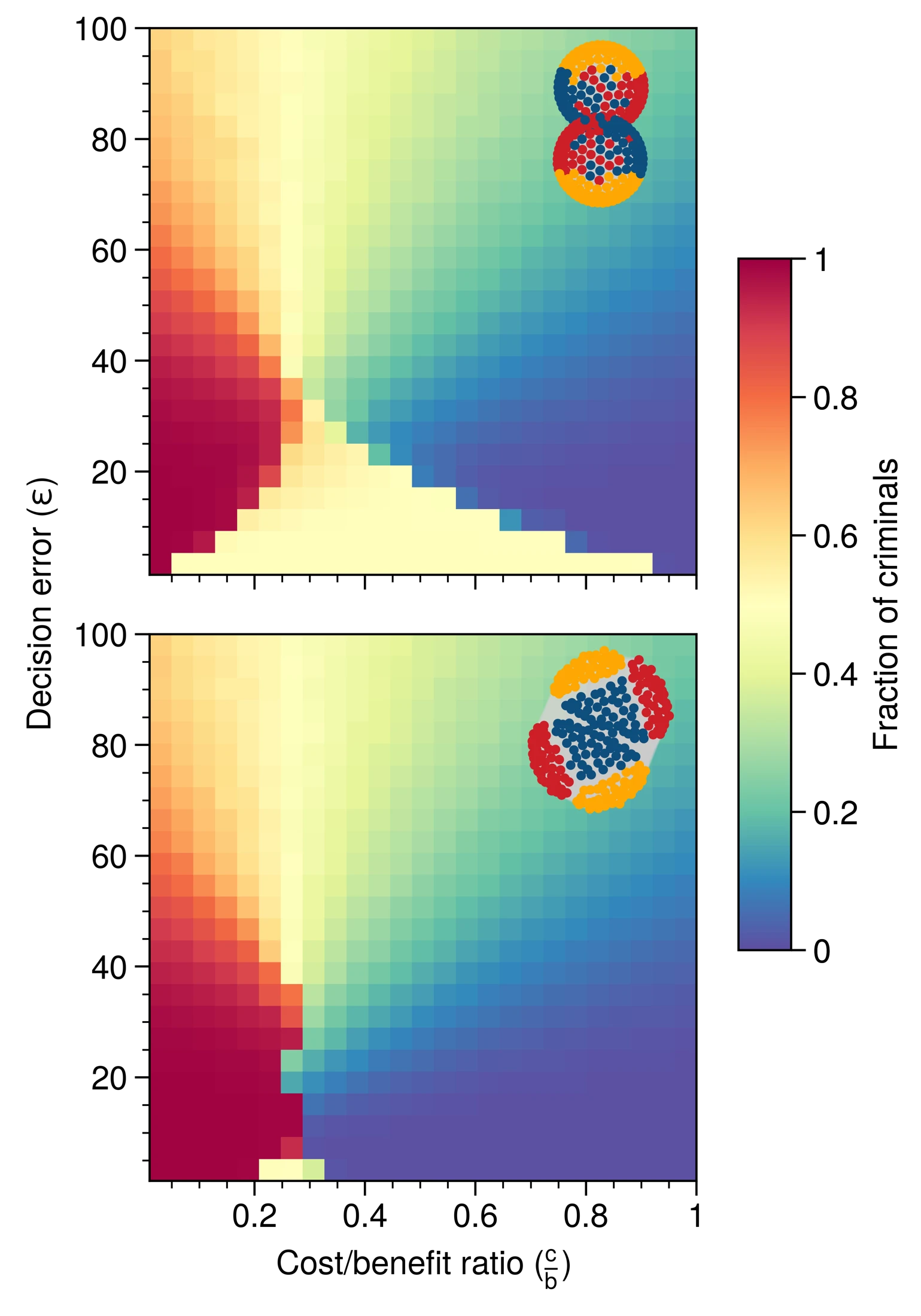
We investigate the importance of these indirect connections by generating two organizations, one criminal and one non-criminal. By varying the connectivity between the two organizations, we expect that there exists some threshold value of cost/benefit and noise for which the non-criminal organization flips to criminal activity. In Section D.IV.1, we observe that the non-criminal organization spontaneously converts to a criminal organization for sufficiently high noise and high benefit. This effect occurs earlier when the number of connections with the criminal organizations increases (Section D.IV.1). The increased connectivity between the two organizations shows how a greater degree of ties between under and overworld can effect the propagation of criminal behavior.

Theories of Organized Crime

I shall not today attempt further to define the kinds of material I understand to be embraced within that shorthand description. But I know it when I see it, and the motion picture involved in this case is not that I know it when I see it - Justice Potter Stewart [247]

Understanding crime can be tackled from multiple perspectives. A theory on crime provides a lens to view the topic. Crime, like any abstract topic, is difficult to define yet easy to recognize. The concept of crime touches upon many different topic such as ethics, morality, the rule of law, philosophy, and psychology to name a few. To merely list the plentiful theories of crime would make the discussion that follows too broad and unbearable. We therefore want to focus on a narrower topic: organized crime.

Organized crime differs itself from other forms of crime by its adjective. The crime is not merely any crime, it is organized. The addition of this word invokes imagery of motor gangs, Mafia, and cartels, but less so of the ordinary thief. However, organized crime usually refers to something more than merely a criminal act that was performed. A burglary that is prepared is therefore not necessarily considered to be organized crime. What then is this organized crime?

Why is it important to define organized crime? Organized crime encompass many different aspects of society that are difficult to grasp in its entirety. Surely any definition of crime will fall short of what organized crime is [120], [121]. The concept of what is considered criminal may change over time demanded by changes in society. However, a definition will form a stepping stone towards understanding the problem that law enforcement aim to reduce. That is, by discussing the topic, and reviewing different perspectives, we aim to come closer to a truth at least temporarily. The truth is not in the sense of some Platonian Idea, but rather a workable form that describes adequately the topic of interest.

A definition may aid in the formation of new policy and or laws, and is therefore crucial for computational scientists to align ourselves with a form that warrants computational investigations. It prevents “conceptual puddings” where stereotypes gain a strong footholds and forces us, the scientists, to center around assumptions that inform our models.

After delving into the etymology we will discuss theories influencing the current work. See for a more comprehensive overview [123].

Etymology of Organized Crime

The term “organized crime” began to gain prominence in the early 20th century, particularly in the United States. It became more commonly used during the Prohibition era, which lasted from 1920 to 1933, when the production, sale, and distribution of alcoholic beverages were prohibited by the 18th Amendment to the U.S. Constitution.

During this period, criminal organizations, such as the Italian-American Mafia and other groups, were heavily involved in illegal alcohol production and distribution, as well as other criminal activities. The activities of these criminal organizations and their structured, coordinated nature led to the popularization of the term “organized crime” to describe their activities.

Since then, the term has been used to refer to various forms of criminal enterprises and activities that involve structured, coordinated, and often transnational criminal organizations. It has become a widely recognized concept in criminology, law enforcement, and legal discussions.

Illicit Enterprise Theory

Criminal organizations show remarkable similarity with legal organizations [123]. To commit a criminal act often requires different skills and expertise working together to obtain profit. Indeed some law enforcement strategies focus on mapping the criminal value chains, disrupting the ability of the criminal organization to execute their activities [132], [133].

The value chain includes all roles or activities that support the primary activities bringing a raw resource or service to market [248], human resource management, research and development, firm infrastructure and so on. The value chain describes the business process or coarse steps that make up the business.

For a criminal organization, may include roles or services that do not occur in licit business. For example, strong-arms or murders for hire could be employed to ensure the market position of a criminal organization within the criminal infrastructure. Similarly, logistic roles such acquiring a getaway care may require carjackers to acquire the vehicles.

In short, illegal enterprise theory states that criminal organizations share more similarities than differences with licit businesses. Members of criminal behaviors use rationale and planning to further business endeavors.

Social Embededness of Criminal Networks

A network in general is used to represent data. As such it requires a filter on the meaning of the nodes and edges in the network. For a social network this could be contact, kinship, geographical distance and so on. The interpretation and meaning of social network analysis is therefore highly context dependent.

For a given representation of a social network, other subnetworks can be identified. Consider, for example, a network formed from contact data. Within this social network different subnetworks can be identified. The network of work colleagues is embedded on this social network, similar to friend networks, or kinship networks. The concept of social embedding gains its origins from social economy [249]. Sociologists identified that economic transactions are embedded within the networks of personal relations. Criminal networks, therefore, are another form of embedding [123].

The general idea is that criminal opportunity is formed through social relations. Social relations do not happen at random but often abey the laws of social an geographic distance [250]. The closer people live, the more daily activity people have in common, the less social distance between them. This results in a clustering of people based on factors such as geographic distance, ethnicity, education, age, membership of a local sports club and so on. This aspect is also found in criminal networks [251].

The important point is that for a given observed network structure, the structural position influences the embededness of an individual to be exposed to criminal activity. The network is not a final state, but the snapshot of the outcome of a complex adaptive process that continuously evolves. To understand how some networks thrive while others falter, requires understanding the relationship between the individuals and the kind of dynamics that exists between them.